
Z-FLoc
참고 논문을 찾아보니 매우 인상적이어서 읽어본 논문이다.
이 논문이 인상적인건, 학습을 최대한 자제한 상태에서, Zero-Shot에 포커스를 두었다는 부분과,
가장 최근 논문답게 관련연구들이 잘 정리되어있다. 그 부분이 인상적이다.
Intro
초록을 읽어보면 핵심 문구가 눈에 들어온다.
geometric primitives…… we extract these primitives from bird’s eye view(BEV) projection of monocular 3D reconstrucions …. match them to floorplan via dedicated minimal solvers……..
즉, RGB 이미지를 이용해 3차원 공간을 재구성하고(monocular 3D reconstructions), 그걸 2차원으로 압축하고(BEV), 여기서 직선과 원을 뽑아낸 뒤, 별도의 solver를 이용해 2D CAD도면(floorplan)과 매칭을 수행하여 Global localization을 수행한다는 것이다.
그 외에 이런 저런 말들이 많이 작성은 되어있는데 논문의 서문 특성상 개념적인 말들이 있는 것이니 크게 눈이 가지는 않는다.
어쨌든 이 연구를 통해 Zero-shot 상태에서 데이터셋을 학습하지 않고서도 localization을 가능케 한다고 하는데, LaLaLoc 과 같은 Indoor-2D CAD VPR 분야의 트렌드와 미묘하게 다른 부분이 있다.
Related work
이 논문에서 제법 눈에 들어오는 분야는 Related work부분에서 전체 분야에 대한 정리가 잘되어있고, 장단점을 잘 정리하고 있어서 눈길이 간다.
이 논문에서 소개하고 있는 Related work들은 다음과 같다.
| 논문 약칭 | 요약 | 논문 citation |
|---|---|---|
| LaLaLoc | 파노라마 이미지와 floorplan에서 생성한 layout 표현을 각각 feature로 임베딩하고, 두 모달리티를 공통 latent space에서 비교하여 위치를 추정한다. RGB 이미지와 floorplan 사이의 modality gap을 학습된 feature space로 해결하는 대표적인 learning-based floorplan localization 방법이다. | Howard-Jenkins, H., Ruiz-Sarmiento, J.-R., Prisacariu, V.A., “LaLaLoc: Latent Layout Localisation in Dynamic, Unvisited Environments,” ICCV, pp. 10107–10116, 2021. |
| LaLaLoc++ | LaLaLoc을 확장하여 camera/ceiling height를 알고 있어야 한다는 가정을 제거한다. 전체 floorplan을 직접 feature space에 embedding하여 query image와 비교하며, 새로운 환경의 floorplan에 대한 localization을 수행한다. | Howard-Jenkins, H., Prisacariu, V.A., “LaLaLoc++: Global Floor Plan Comprehension for Layout Localisation in Unvisited Environments,” ECCV, 2022. |
| F3Loc | 일반 perspective RGB image로부터 floorplan과 직접 비교 가능한 1D depth ray를 예측한다. Single-view와 multi-view depth prediction을 결합하고, SE(2) histogram filter를 사용하여 시간에 따른 observation을 누적한다. Z-FLoc에서는 learned observation model + sequential filtering 계열의 대표 방법으로 언급한다. | Chen, C., Wang, R., Vogel, C., Pollefeys, M., “F3Loc: Fusion and Filtering for Floorplan Localization,” IEEE/CVF Conference on Computer Vision and Pattern Recognition (CVPR), 2024. |
| Semantic Rays | F3Loc의 depth-ray 기반 localization을 확장하여 wall, window, door 등의 semantic ray를 함께 예측한다. Depth와 semantic information을 하나의 structural-semantic probability volume으로 결합하여 반복적인 floorplan 구조에서 발생하는 localization ambiguity를 줄인다. | Grader, Y., Averbuch-Elor, H., “Supercharging Floorplan Localization with Semantic Rays,” Proceedings of the IEEE/CVF International Conference on Computer Vision (ICCV), pp. 27116–27125, 2025. |
| PF-Net | Particle filter의 motion model과 observation model을 neural network와 결합하여 differentiable particle filtering을 수행한다. 이미지와 map patch 사이의 learned similarity를 observation likelihood로 사용하며, sequential observation을 이용해 pose distribution을 갱신한다. | Karkus, P., Hsu, D., Lee, W.S., “Particle Filter Networks with Application to Visual Localization,” Conference on Robot Learning (CoRL), 2018. |
| C3Po | DUSt3R를 활용하여 서로 다른 view와 modality 사이의 point-level correspondence를 학습한다. Image와 floorplan 사이의 correspondence를 얻은 뒤 localization을 geometric registration 문제로 변환한다. 즉 correspondence 추정은 learning에 의존하지만 최종 pose 계산은 geometric registration으로 접근한다. | Huang, K.-W., Li, B., Hariharan, B., Snavely, N., “C3Po: Cross-View Cross-Modality Correspondence by Pointmap Prediction,” Advances in Neural Information Processing Systems (NeurIPS), Vol. 38, 2025. |
| FloorplanNet | LiDAR에서 생성한 occupancy map과 floorplan을 graph representation으로 표현하고, graph neural network를 이용하여 두 지도를 matching한다. Geometry를 사용하지만 map matching 자체가 학습 기반이라는 특징이 있다. | Feng, D., He, Z., Hou, J., Schwertfeger, S., Zhang, L., “FloorplanNet: Learning Topometric Floorplan Matching for Robot Localization,” IEEE International Conference on Robotics and Automation (ICRA), pp. 6168–6174, 2023. |
| SeDAR | Depth 대신 CNN이 예측한 semantic label을 observation으로 사용한다. Semantic 정보를 floorplan과 비교하고 Monte Carlo Localization을 수행하여 카메라 위치를 추정한다. 순수 geometry만 사용하는 방법과 달리 semantic scene understanding을 localization cue로 활용한다. | Mendez, O., Hadfield, S., Pugeault, N., Bowden, R., “SeDAR: Reading Floorplans Like a Human – Using Deep Learning to Enable Human-Inspired Localisation,” International Journal of Computer Vision, Vol. 128, No. 5, pp. 1286–1310, 2020. |
| SPVLoc | Texture가 없는 3D semantic model에서 semantic panorama를 렌더링한 뒤, query perspective image의 embedding과 rendered panorama의 embedding을 matching한다. Semantic rendering을 이용해 perspective image와 구조적 map 사이의 modality gap을 줄인다. | Gard, N., Hilsmann, A., Eisert, P., “SPVLoc: Semantic Panoramic Viewport Matching for 6D Camera Localization in Unseen Environments,” ECCV, 2024. |
| OrienterNet | 입력 이미지로부터 neural BEV representation을 예측하고 이를 OpenStreetMap과 neural matching하여 2D 위치와 orientation을 추정한다. 실내 floorplan보다는 outdoor public map localization을 대상으로 하지만, egocentric image를 BEV로 변환한 뒤 overhead map과 정합한다는 점에서 관련된다. | Sarlin, P.-E., DeTone, D., Yang, T.-Y., Avetisyan, A., Straub, J., Malisiewicz, T., Rota Bulò, S., Newcombe, R., Kontschieder, P., Balntas, V., “OrienterNet: Visual Localization in 2D Public Maps with Neural Matching,” CVPR, 2023. |
| Spatial Graph-based Localization | LiDAR-derived map과 scaleless floorplan 사이에서 SIFT feature를 matching하고 similarity transformation을 추정한다. 별도의 학습이 필요 없는 training-free 방식이지만, 충분히 정확하고 넓은 영역을 커버하는 LiDAR point cloud를 필요로 한다. | Ewe, Z.L., Chang, F.H., Huang, Y.S., Fu, L.C., “Spatial Graph-based Localization and Navigation on Scaleless Floorplan,” IEEE Robotics and Automation Letters, Vol. 9, No. 4, pp. 3932–3939, 2024. |
| 2D Map Alignment | Occupancy map을 영역(region) 단위로 분해하고 room/region 구조를 이용하여 두 2D map을 정합한다. Handcrafted geometric representation을 이용하기 때문에 별도의 학습은 필요 없지만, room geometry가 충분히 완전하게 관측되어야 한다. | Gholami Shahbandi, S., Magnusson, M., “2D Map Alignment with Region Decomposition,” Autonomous Robots, Vol. 43, 2019. |
| Area Graph Matching | Occupancy map에서 공간을 영역 단위의 graph로 표현한 뒤 area graph 사이의 구조적 correspondence를 찾아 map을 정합한다. Training-free이지만 안정적인 room/area structure를 생성할 수 있을 정도의 고품질 map을 필요로 한다. | Hou, J., Yuan, Y., He, Z., Schwertfeger, S., “Matching Maps Based on the Area Graph,” Intelligent Service Robotics, Vol. 15, No. 1, pp. 69–94, 2022. |
| FGPL | Fully Geometric Panoramic Localization. Panorama에서 추출한 2D line과 사전에 구축된 3D line map의 geometric relationship을 사용한다. Line distance field와 line intersection을 이용해 pose candidate를 탐색한 뒤 primitive 기반 refinement를 수행한다. Learned visual descriptor가 필요 없고 generalization이 강하지만 panorama와 정확한 height 정보가 요구된다. | Kim, J., Jeong, J., Kim, Y.M., “Fully Geometric Panoramic Localization,” Proceedings of the IEEE/CVF Conference on Computer Vision and Pattern Recognition (CVPR), 2024. |
| PALMS+ | Off-the-shelf monocular depth foundation model을 사용하여 여러 RGB 이미지로부터 scale-aligned point cloud를 복원한다. 이를 BEV로 투영한 뒤 floorplan과 convolution/correlation 방식으로 비교하여 pose posterior를 구한다. 별도 localization training은 필요 없지만 하나의 고정된 위치에서 360° 전체를 촬영해야 한다. | Cheng, Y., Princen, B., Manduchi, R., “PALMS+: Modular Image-Based Floor Plan Localization Leveraging Depth Foundation Model,” arXiv:2511.09724, 2025; accepted to IEEE/CVF Winter Conference on Applications of Computer Vision (WACV) 2026, Application Track. |
이걸 특징별로 다시 구분해보면 다음과 같다.
| 계열 | 대표 연구 | 핵심 접근 | Z-FLoc이 지적하는 한계 |
|---|---|---|---|
| Learning-based cross-modal matching | LaLaLoc, LaLaLoc++ | Image와 floorplan을 공통 feature space에서 비교 | Domain-specific training 필요 |
| Learning + Sequential Filtering | F3Loc, PF-Net, Semantic Rays | Learned observation likelihood를 시간에 따라 누적 | 학습 데이터 및 domain generalization 문제 |
| Learned Correspondence | C3Po | Image-floorplan point correspondence를 학습한 뒤 geometric registration | Correspondence 생성이 learned model에 의존 |
| Semantic Localization | SeDAR, SPVLoc | Semantic label 또는 semantic rendering을 활용 | Semantic model/annotation 및 학습 필요 |
| Neural BEV Matching | OrienterNet | Image에서 BEV를 예측하고 overhead map과 neural matching | Learned representation에 의존 |
| Training-free Map Alignment | Spatial Graph, 2D Map Alignment, Area Graph | LiDAR/occupancy map을 floorplan과 geometric matching | 정확하고 coverage가 높은 point cloud 필요 |
| Fully Geometric | FGPL | Line 및 line intersection으로 pose search/refinement | Panorama와 정확한 height 정보 필요 |
| Foundation Depth + Dense BEV Matching | PALMS+ | Monocular depth → point cloud → BEV → floorplan correlation | 고정 지점에서 360° observation 필요 |
| Z-FLoc | Z-FLoc | RGB sequence → 3D reconstruction → BEV → line/circle → hybrid RANSAC | Training-free이면서 partial/noisy observation을 다루는 것을 목표로 함 |
나름 자료검색 많이 했다고 생각했는데, 이걸 보니 또 읽어봐야 할 것이 몇가지 더 있다. C3Po도 그렇고, SeDAR도 있네…. 하.. 분야가 점점 커진다.
Zero-Shot Floorplan Localization
문제 정의
연속된 RGB이미지가 주어진다. 이 이미지들의 카메라 포즈(SE(3)) 와 카메라 내부값(intrinsic)도 같이 주어진다. 이걸 토대로 SE(2)인 2D 캐드도면상의 Pose를 찾는 것이다.
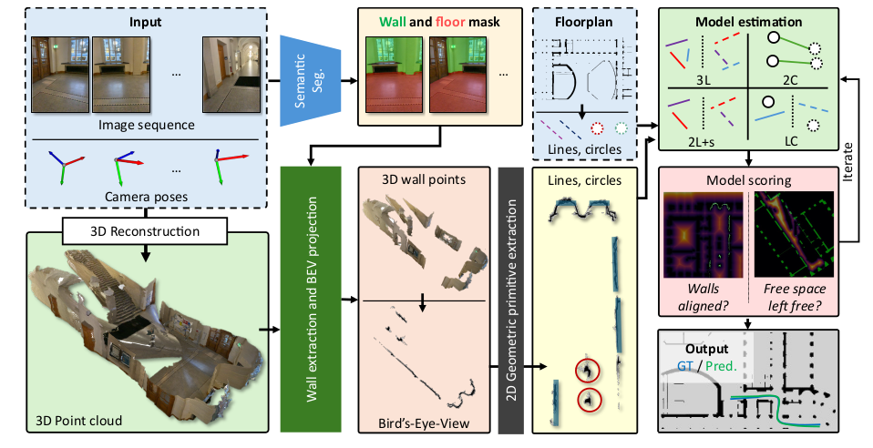
전체 pipeline 이미지에서 이런 과정을 간략히 보여주고 있다.
Input 데이터에 대해, 3차원 공간 재구성을 하는 라인과, 이 이미지에서 객체 인식을 통해 벽과 바닥을 구분해내고, 이걸 재구성된 3차원 공간에 적용시켜 벽 정보만 추출, 이걸 Top-view 로 변환한다. 여기서 나온 선과 원을 추출하여 FloorPlan의 원과 선들과 매칭시키는 작업을 수행하는데, 이때 Model estimation이 논문에서 말하는 Solver다. 그리고 그 문제를 풀기위한 Objective function이 Model scoring이라는 이름으로 정리되어있다. 이를 통해 위치를 추정하고 location과 trajectory를 추정해낸다.
천천히 톺아보자.
사용된 Foundation 모델
이 논문에선 두가지 모델을 사용한 것이 눈에 띈다. 그걸 시작으로 전체 파이프라인을 순서대로 번호를 매겨보자.
1) RGB 이미지와 카메라 포즈정보가 입력된다. 2-1) 이미지 정보를 토대로 3차원으로 재구성한다. (MapAnything) 2-2) 원본 이미지 정보에서 벽과 바닥정보를 구분해 픽셀에 라벨링한다.(Mask2Former) 3) 3D PCD 맵에서 벽만 추출한 다음 BEV로 변환한다. 4) FloorPlan과 BEV View에서 primitives(선, 원) 성분을 추출해낸다. 5) 추출된 Primitives를 4개의 Solver를 이용해 비교하면서 RANSAC 알고리즘을 이용해 반복한다(iteration) 6) iteration을 통해 좀더 지지를 많이 받는 pose를 최종 가설로 선택한다.
우선 사용한 모델에 대해 먼저 실습해본다.
1. 입력정보
앞서 서술했듯이 RGB 이미지 시퀸스를 사용하는데, 거기에 더해 각 프레임의 상대 카메라 Pose정보 (SE(3)), 카메라 intrinsic 정보가 모두 주어진다.
상대 Pose만 가지고 있기때문에, 나중에 중력추정을 해서 보정하는 작업을 거쳐야 한다.
그리고 이 정보와 Sync를 맞추기 위해 2D 건축 캐드도면(floorplan)이 필요하다.
이러한 입력정보를 가지고 있는 데이터셋이 필요하다. 논문에선 평가용으로 다음과 같은 데이터셋을 사용했다.
| Dataset | 유형 | 특징 | Z-FLoc 관점 |
|---|---|---|---|
| Gibson(t) | Synthetic indoor | 작은 실내, upright camera, 넓은 FOV | 비교적 정형적인 wall geometry |
| LaMAR HGE | Real-world indoor | 대형 대학 건물, occlusion 많음, narrow FOV | 복잡하고 cylindrical structure도 존재 |
| LaMAR CAB | Real-world indoor | HGE와 다른 건물 | cross-building generalization 평가 |
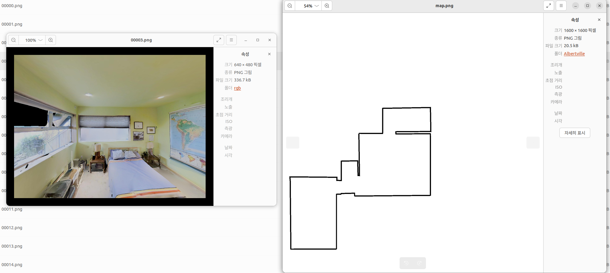
일단 Gibson 데이터셋을 받아서 봤는데 합성데이터란걸 받아보고 나서야 알았다..
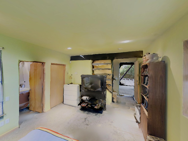
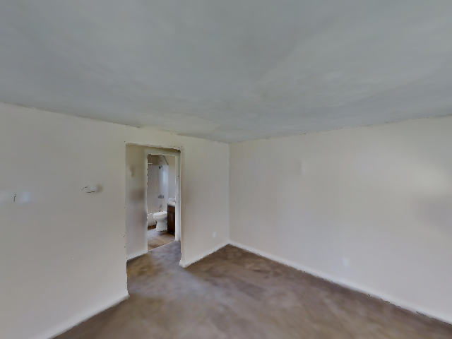
근데… 이렇게 우글우글거리는건 좀 심하지 않나..?
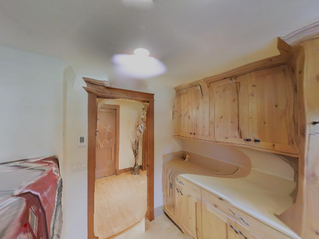
각 폴더에 이미지정보와 카메라 포즈정보, 그리고 맵정보도 이렇게 다 같이 들어가있으니 처음 알고리즘 연습해보기엔 좋은 자료인듯 하다.
2-1. 이미지정보를 토대로 3차원 재구성하기
이 논문에서는 들어오는 이미지 정보를 MapAnything을 통해 3차원으로 재구성한다. 사실 RGB-D를 사용한다거나, 다른 Vision SLAM의 기법들을 사용한다면 다른 대안도 있을텐데 굳이 foundation model 계열의 3차원 재구성방식을 사용한다. 장단점에 대해 고민해볼 여지가 있다.
MapAnything은 한 장 이상의 RGB 이미지와 선택적인 calibration·depth·camera pose를 받아 metric 3D geometry와 camera를 한 번의 feed-forward 추론으로 예측한다. image-only 입력에서도 다음 요소를 함께 추정한다.
- 픽셀별 depth와 camera ray
- view별 camera pose
- 장면의 metric scale
- camera/world frame의 dense point map
그 말인즉슨, Pose정보를 주지 않아도 돌아가긴 한단 소리. 물론 정확도/정밀도의 문제는 발생하겠지만.
여기서 MapAnything의 상세한 디테일을 들여다보지는 않겠다. 그건 별도의 칸을 들여 리뷰해볼 사항이다. 여기선 활용방식에 대해 좀 더 파보자.
핵심 입·출력
MapAnything API는 list[view dict]를 입력받아 같은 순서의 list[prediction dict]를 반환한다. 이때 batch 차원 B와 view 개수 N은 다르다.
입력
| 키 | 전처리 후 shape | 의미 |
|---|---|---|
img |
(B, 3, H, W) |
DINOv2 방식으로 정규화된 RGB |
data_norm_type |
보통 ["dinov2"] |
encoder 정규화 정보 |
지금은 image-only로 진행했다. load_images(...)가 resize/crop, 정규화, batch 차원 생성을 담당한다. 선택적으로 intrinsics (3,3), depth_z (H,W), OpenCV cam2world (4,4) pose를 넣을 수 있지만 Albertville의 poses.txt와 depth40.txt는 이 형식이 아니다. Pose.txt 는 2D 좌표값과 Yaw 값이 으로 나와있어 3차원정보로 변환의 필요성이 있고, depth40.txt는 일종의 GT자료로 활용하는 데이터다. 간편하게 재현해보기 위해 여기선 이미지만 사용하여 수행한다.
주요 출력
| 키 | shape | 의미 |
|---|---|---|
pts3d |
(B,H,W,3) |
공통 world frame의 픽셀별 3D point |
pts3d_cam |
(B,H,W,3) |
해당 camera frame의 3D point |
depth_z |
(B,H,W,1) |
camera optical axis 기준 Z-depth |
camera_poses |
(B,4,4) |
OpenCV 축의 cam2world pose |
conf |
(B,H,W) |
상대적인 픽셀별 confidence |
mask |
(B,H,W,1) |
후처리가 적용된 유효 픽셀 mask |
img_no_norm |
(B,H,W,3) |
시각화 및 point color용 RGB |
metric_scaling_factor |
(B,) |
예측에 적용된 metric scale |
주요 구현 코드
전체 코드는 조금 길고, MapAnything 의 핵심 코드들만 추려본다.
import torch   #뭐, 이건 필수고. 결국 GPU가속을 사용해야 한다.

from mapanything.models import MapAnything
from mapanything.utils.image import load_images

device = "cuda" if torch.cuda.is_available() else "cpu"


model = MapAnything.from_pretrained(
    "facebook/map-anything"
).to(device).eval()

views = load_images(["00000.png", "00001.png"...........]) #예시코드다.

with torch.inference_mode():
    predictions = model.infer(views)

points_3d = predictions[0]["pts3d"]
depth = predictions[0]["depth_z"]
camera_pose = predictions[0]["camera_poses"]
만약 입력할 pose정보가 있다면 views 의 입력부분은 이렇게 바꾸면 된다.
views = preprocess_inputs([{"img": image, "intrinsics": K, "camera_poses": T_c2w}])
sim(3) 정렬 추가
MapAnything을 통해 나온 결과를 실제 좌표계에 맞추는 후처리가 필요하다.
\[\mathbf{p}_{world}=sR\mathbf{p}_{pred}+t\\]아마 논문에서도 이 수식이 나올텐데, 겁먹지 말자. 전형적인 수식이고, 리군연산의 형태다.
이미지를 통해 추정한 point cloud들을 정렬해야 한다. 이것도 sim3만 따로묶어서 주제로 다루어야 할 정도이니, 여기선 간단하게 활용예제정도만 놓고 보자.
scale, R, t = estimate_sim3(points_pred, points_ref)
points_aligned = scale * (points_pred @ R.T) + t
정말 심플하다.
전체 이미지에 대한 추론, 정렬, 병합 반복
여러장의 이미지가 들어가게 되면, 추론, 정렬, 병합을 반복해서 수행해야 한다.
# 1. 추론
pred_ref = model.infer(preprocess_inputs(views_ref))
...
pred_new = model.infer(preprocess_inputs(views_new))

# 2. 정렬: 겹치는 대응점으로 Sim(3) 계산
scale, R, t = estimate_sim3(correspondences_new, correspondences_ref)
points_new_aligned = scale * (points_new @ R.T) + t

# 3. 병합
points_merged = np.concatenate([points_ref, points_new_aligned], axis=0)
그러나 한번에 모든 이미지를 넣게 되면 GPU메모리가 남아나질 않으니, 이미지를 묶어서 넣는 방법을 선택한다. 이렇게 넣는걸 chunk라고 한다. 여기서는 window 라는 이름으로 수행했다. sliding window에서 따온것이라 그러려니 하자. 아래 코드는 실제 동작되는건 아니고, 수행했던 예제에서 요약한 것이다.
for start, end in window_ranges:
    predictions = model.infer(views)  # 1. 현재 window 추론

    source, target, _ = collect_overlap_correspondences(
        current_frame_ids, predictions, alignment_references
    )
    scale, R, t, _, rmse = robust_similarity_alignment(source, target)  # 2. 정렬

    global_points = transform_points(local_points, scale, R, t)

    if frame_id not in processed_frames:
        point_chunks.append(global_points)  # 3. 병합
이걸 수행해서 matplot으로 확인해보면 아래와 같다.
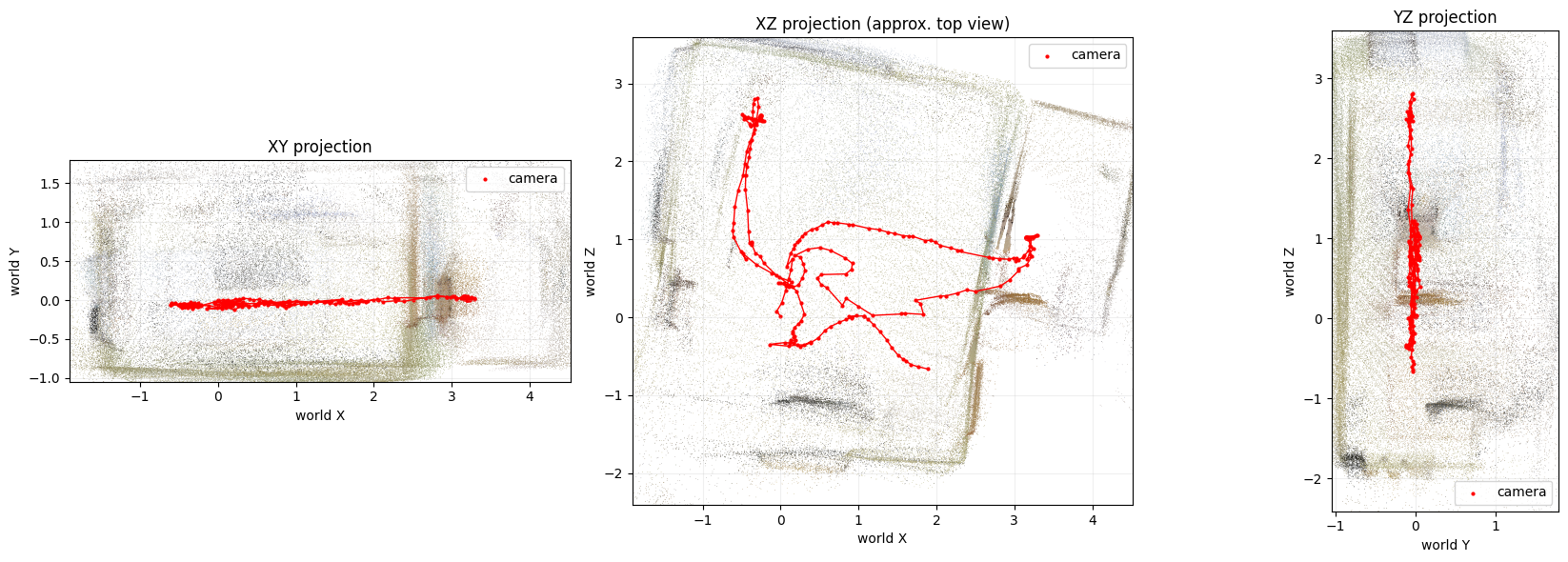
이미지를 chunk로 핸들링하면서, drift등이 발생하는데, 이걸 줄이기 위해서 오배 이제, 이 포인트 클라우드들에서 벽과 바닥정보를 구분해보자.
2-2. 이미지 정보에서 벽과 바닥정보를 구분해 픽셀에 라벨링
이 논문에서는 Mask2Former를 사물 인식의 수단으로 사용하고 있다.
다른 방법들도 있는데, 굳이 꼭 이것이어야 하나 하는 생각도 들긴 한다. 특히나 실시간성에서 제약이 많이 올 것 같은데.(여기에 대해선 YOLO-seg 시리즈가 대안이긴 하나, 막상 써보면 약간 부정확할때가 있다.)
아마도 정확도를 확보하기 위해 Mask2Former를 사용한 것으로 생각된다.
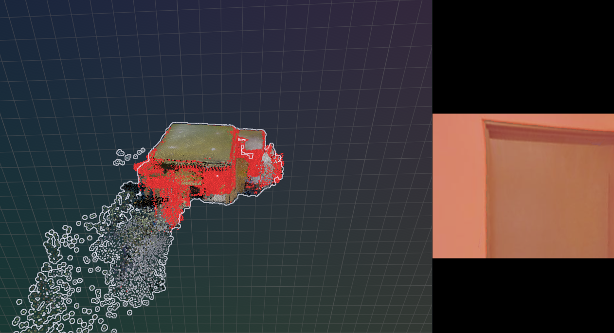
어쨌거나, Mask2Former를 이용해서 구분할 건 두가지다. “Wall” 과 “floor”인데, Wall의 경우는 2D Floorplan과 정합하기 위한 feature로 사용되고, floor의 경우는 중력방향 보정을 위해서 사용된다.
RGB 이미지를 가지고 depth 추정에, object 추정을 해야 하므로, GPU 점유와 해제에 조심해야 한다. 아.. 이건 생각도 못했네. 따라서, 설명은 MapAnything을 먼저 이야기했지만, 실행은 RGB이미지가 들어온 다음 Mask2Former를 먼저 수행한 후, GPU 메모리 점유를 해제하고 MapAnything으로 넘어가야 한다.
논문에선 어떤 Backbone을 썼는지 밝히진 않고 있다. 따라서, wall이 클래스로 제공되는 범용 모델인 ADE20K 중 GPU에 무리없는 작은 모델로 선정한다. 필수 라이브러리들을 포함하여 설정하는 것은 다음과 같다.
import torch
import numpy as np
import matplotlib.pyplot as plt

from PIL import Image
from transformers import (
    AutoImageProcessor,
    Mask2FormerForUniversalSegmentation,
)

MODEL_NAME = "facebook/mask2former-swin-small-ade-semantic"

processor = AutoImageProcessor.from_pretrained(MODEL_NAME)

model = Mask2FormerForUniversalSegmentation.from_pretrained(MODEL_NAME)

device = torch.device("cuda" if torch.cuda.is_available() else "cpu")

model = model.to(device)
model.eval()
Wall 과 Floor가 어떻게 설정되어있는지 확인해보자.
for class_id, class_name in model.config.id2label.items():
    if (
        "wall" in class_name.lower()
        or "floor" in class_name.lower()
    ):
        print(class_id, class_name)


# 반드시 위의 출력 결과를 확인해서 지정
WALL_CLASS_ID = 0
FLOOR_CLASS_ID = 3
위의 모델을 가지고 구현하면 다음과 같다. Mask2Former에 RGB 이미지를 그대로 tensor로 넣는 것이 아니라 AutoImageProcessor를 사용한다.
#processor = AutoImageProcessor.from_pretrained(MODEL_NAME) 앞서서 선언한걸 참조하자.

#이미지를 불러오고, device에 올린다.
image = Image.open("example.jpg").convert("RGB")

inputs = processor(images=image, return_tensors="pt",)
inputs = inputs.to(device)

# Mask2Former inference
with torch.no_grad():
    outputs = model(**inputs)

# semantic map 데이터 가져오기.
semantic_map = ( processor
                  .post_process_semantic_segmentation(
                        outputs,                                                               target_sizes=[(image.height, image.width)],
                        )[0]
                )
#Wall mask와 Floor mask 정리하기

wall_mask = (semantic_map == WALL_CLASS_ID).cpu().numpy()

floor_mask = (semantic_map == FLOOR_CLASS_ID).cpu().numpy()
모델을 통해, 이미지에 sementic vector를 부여하면, 이중 Wall에 해당하는지 체크(출력이 Boolean이란 소리다) 해서 결과를 numpy 의 포맷으로 가져온다. 그러면 wall_mask.shape 는 H x W의 크기를 갖는 Binary Mask를 갖는다. 즉, Mask2Former의 output과 MapAnything image와 같은 사이즈가 된다는 뜻이 된다.
MapAnything의 출력은 이렇게 변환된다. (local point의 형태는 색상을 포함하므로, HxWx3 이 된다.)
local_points = prediction["pts3d"][0].detach().float().cpu().numpy()
이걸 이렇게 전개하는 것이다.
points = global_points[::4, ::4]  #local_points에서 카메라 포즈를 반영한 변환식을 거쳐 전체 좌표계로 왔다라고 하자.
mask   = wall_mask[::4, ::4]

wall_points = points[mask]
이걸 단순한 예로 표현해보면, 어떤 이미지에서, u=320, v=180인 지점의 픽셀을 가져오자.
RGB에서 이 픽셀이 벽이라고 한다면, Mask2Former는
wall_mask[180,320] = True
라는 형태로 결과를 저장하게 된다.
MapAnything은 같은 위치에 대해
pts3D[180,320] = [1.37, -0.42, 4.81]
라는 형태의 좌표값을 가지는 출력을 만든다.
이걸 Rerun에 연동해서 화면에 출력해보면 다음과 같다.
3. 벽 확인, Depth정보를 이용한 벽 추출
방금까지는 실습하기 좋은 foundation model을 중심으로 해봤다. 본격적으로 논문을 재현해가면서 한번 톺아보자.
벽면을 구분하는데 문제가 하나 있다. 도면의 표현방법에 있어, 문과 통로가 있는 부분이다. Mask2Former를 했을때 이 부분이 벽으로 보인다면 매칭에 어려움이 발생한다.
아래 도면을 보자. 파란 화살표 부분이 화장실 들어가는 부분이다. (도면이 좌우 반전되어있다…왜?)
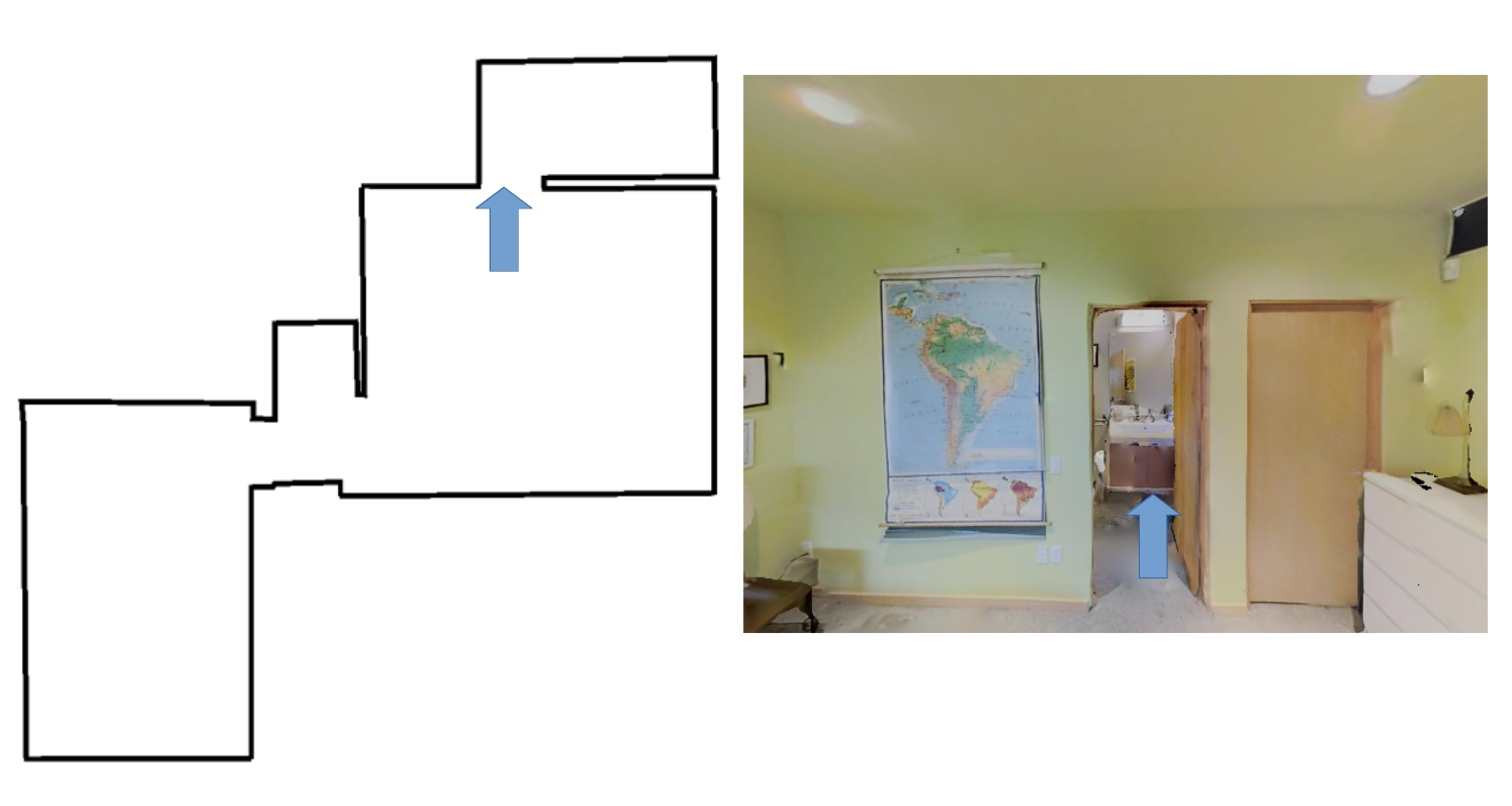
따라서 무턱대고 포인트클라우드에서 벽만 추출할 경우 이런 문 위의 벽들도 같이 BEV에 인식되어 통로와 벽을 구분할 수 없게 되는 사태가 나온다. 근데 굳이 이래야 하나 싶기도 한게… 그냥 2D로 프로젝션해서 일정이상 포인트가 모이지 않으면 그냥 통로로 해도 되지 않나..? 싶은데.. 굳이…? (왜냐면 이거 구현하는 연산이 솔찮이 복잡하다.)
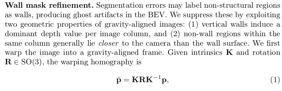
이걸 보정하기 위해서, 중력방향으로 전체 포인트를 변환한다. 일단 기준점 정렬이다. (그걸 Warp 시킨다고 표현하고 있다.) 수식 1은 그걸 말하고 있다. (그냥 포인트 좌표변환한다는 소리니까 너무 겁내지말자.)
그리고, 중력방향으로 보정되어 얻게되는 depth정보는 수식 2라는 뜻이다.
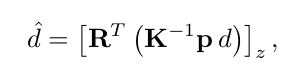
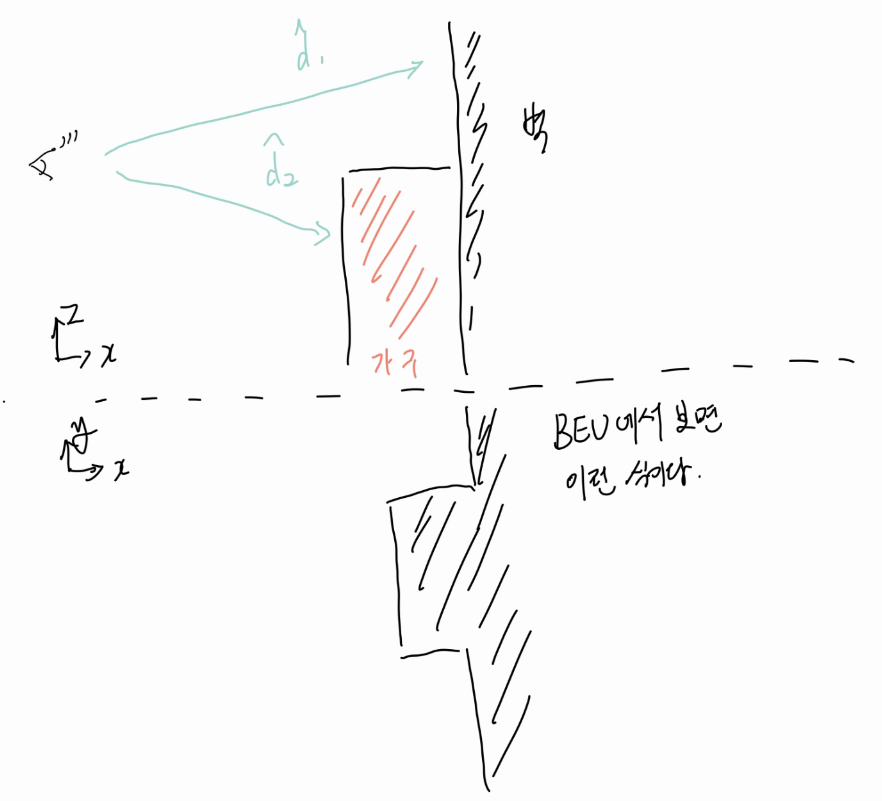
중력의 방향대로 이미지가 정렬되었다면, 수직벽이 임미지에서 가지는 depth정보는 비교적 일정한 값을 가져야 한다. 만약 어떤 픽셀이 해당벽의 깊이보다 더 크다면 그건 벽이 아닐 가능성이 더 큰 셈이다.
따라서, 해당열의 벽 깊이를 $\tilde{d}$ 라 할때, $\tilde{d}$ 는 depth 값들의 중앙값으로 하고,

어떤 열에서 벽이아닌 픽셀의 깊이값이 해당 벽의 깊이보다 더 크다면 그 열 전체가 잘못된 벽 검출일 가능성이 높으므로, 제거한다.

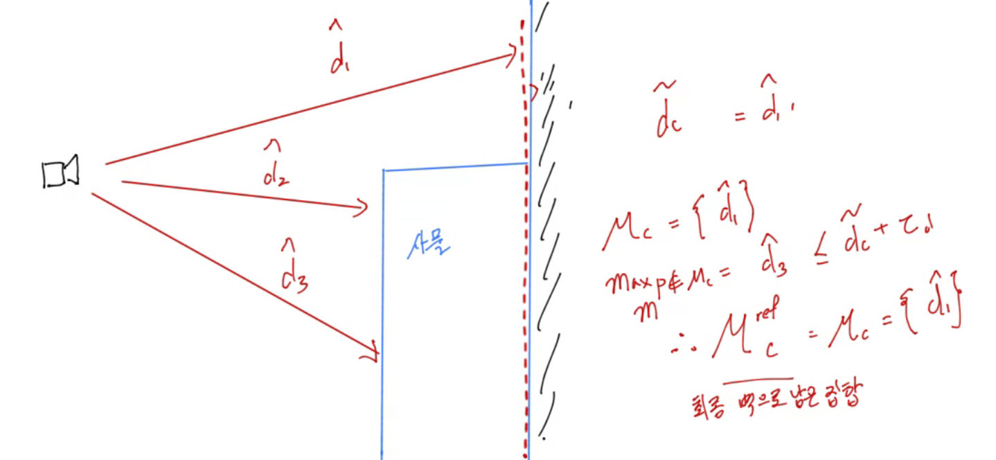
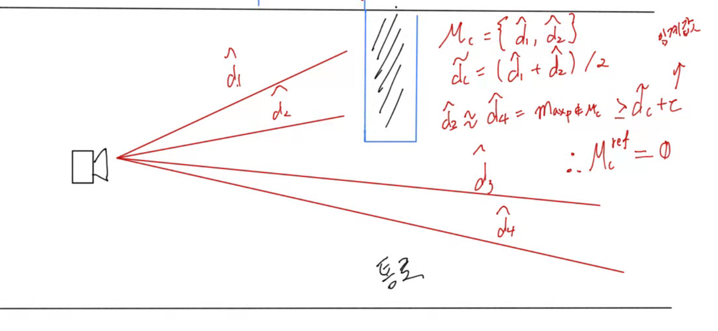
$\tau$ 는 임계값을 나타낸다. $\mathcal{M}_c$ 은 그 열에서 벽이라고 마스킹된 점들의 집합이다.즉, 벽이라고 마킹되지 않았는데, 벽과 큰 Depth 차이가 나지 않는다면, 그냥 벽으로 덮어씌운단 소리고. 만약 뻥 뚫린 통로같은게 있으면 제외한다는 의미다. 그 점의 detph값은 median값+임계값 보다 작아야 한다. 따라서 아래 그림처럼의 경우는 문제가 없다.
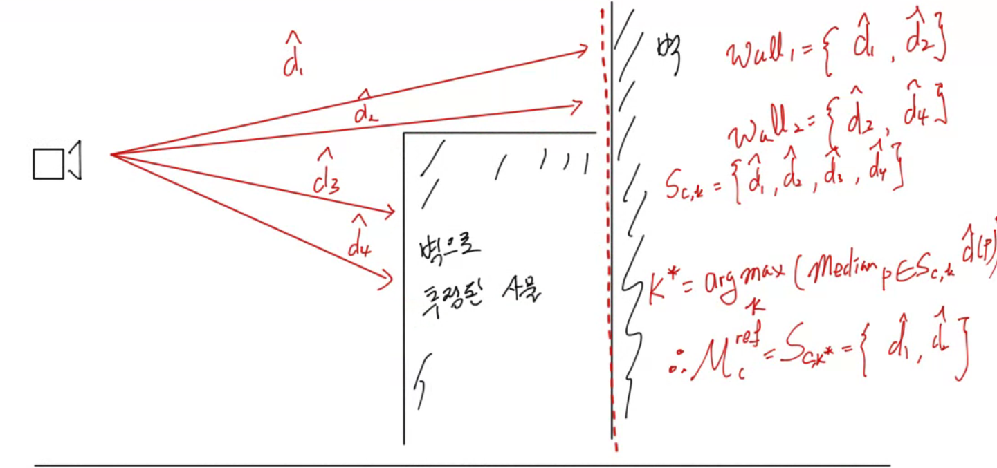
또한, 한 열에 여려개의 wall instance가 있다면, 가장 멀리 있는 wall segment만 유지한다. 수식 5의 내용을 풀어보면 그렇다.

이 조건들을 그림으로 다시 그려보면 이렇다. 수식 (3)과 수식 (4)의 개념은 다음과 같다.
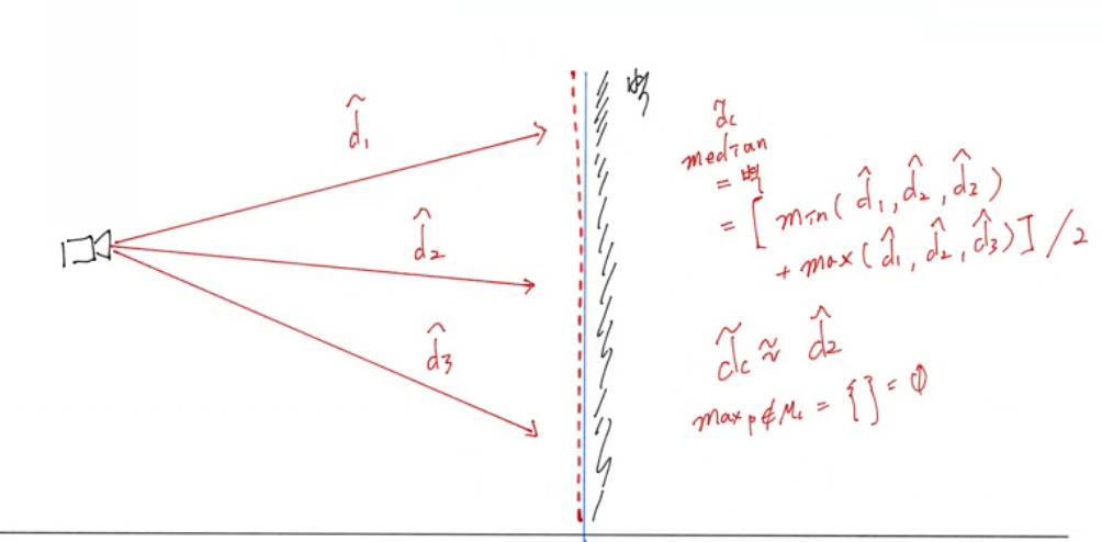
장애물로 가려진 벽이 존재한다면 이런식으로 대응된다.
하지만, 문이나 통로로 인해 뚫린 곳이라면 벽으로 인정하지 않는다.
그리고 수식 (5)의 개념을 반영하면, 다음과 같다.
이걸 구현한 코드부분을 보자.
Gravity 확인
1) 우선 바닥이라 인지된 부분의 중심점을 찾는다. 2) 중심점을 기준으로 PCA 주성분을 찾는다. 3) 이 값을 바탕으로, 평면방정식 $n^\top x + d = 0$ 의 파라미터를 찾는다.
def fit_floor_plane_pca(points: np.ndarray, camera_centers: np.ndarray)
    points = np.asarray(points, dtype=np.float64)

    # Floor point cloud의 가장 작은 PCA 축은 바닥 평면의 법선이다.
    centroid = points.mean(axis=0)
    centered = points - centroid  #잔차 Residual을 구하고,
    covariance = centered.T @ centered / len(points)  #공분산을 계산한 다음
    eigenvalues, eigenvectors = np.linalg.eigh(covariance)  #고유값을 구하자.
    normal = eigenvectors[:, np.argmin(eigenvalues)]  #그러면 법선 벡터를 구할 수 있다.

    # 법선의 부호 모호성을 없앤다. camera에서 floor 쪽을 향하는 방향을 gravity-down으로 선택한다.
    camera_center = np.median(camera_centers, axis=0)
    if np.dot(normal, centroid - camera_center) < 0:
        normal = -normal
    gravity_down = normal / np.linalg.norm(normal)  #평면 방정식의 파라미터 n에 해당
    plane_offset = -float(np.dot(gravity_down, centroid))  #평면 방정식의 파라미터 d에 해당
    residuals = centered @ gravity_down  # 평면이 잘 놓였는지 알 수 있는 지표

    return {
        'centroid': centroid,
        'covariance': covariance,
        'eigenvalues': eigenvalues,
        'gravity_down': gravity_down,
        'plane_offset': plane_offset,
        'residuals': residuals,
    }
refine coulumns
정렬된 벽줄을 어떻게 분류해내는가에 대한 함수다.
def refine_aligned_columns(
                              wall_mask: np.ndarray,
                              aligned_depth: np.ndarray,
                              valid_mask: np.ndarray,
                              tau_d: float,
                              segment_depth_gap: float,
                            )
    # 출력은 raw semantic wall의 부분집합이다. 새 wall을 만들지 않고 신뢰하기 어려운
    # wall pixel만 제거한다.

    # 변수 초기화
    refined = np.zeros_like(wall_mask, dtype=bool)
    finite_positive = valid_mask & np.isfinite(aligned_depth) & (aligned_depth > 0)

    # Upright view에서는 수직 벽이 column별로 거의 같은 depth를 가져, column 단위 검사가 가능하다.
    for column in range(wall_mask.shape[1]):
        wall_rows = np.flatnonzero(wall_mask[:, column] & finite_positive[:, column])
        if len(wall_rows) == 0:
            continue
        wall_depths = aligned_depth[wall_rows, column]
        # Median은 segmentation 경계의 소수 outlier에 덜 민감한 대표 wall depth다.
        representative_depth = float(np.median(wall_depths))
        non_wall = (~wall_mask[:, column]) & finite_positive[:, column]

        # semantic wall보다 충분히 먼 non-wall 구조가 있으면, 이 column의 wall label은
        # 가려진 배경/잘못된 segmentation일 가능성이 높으므로 전부 버린다 (논문 식 4).
        if np.any(non_wall) and float(np.max(aligned_depth[non_wall, column])) > representative_depth + tau_d:
            continue

        order = np.argsort(wall_depths)
        sorted_rows = wall_rows[order]
        sorted_depths = wall_depths[order]

        # 한 column에 서로 다른 깊이의 벽 후보가 있으면 depth gap으로 분할한 뒤,
        # 가장 먼 segment만 남긴다. 가까운 물체/ghost wall보다 실제 배경 벽을 우선한다 (식 5).
        split_locations = np.flatnonzero(np.diff(sorted_depths) > segment_depth_gap) + 1
        segments = np.split(sorted_rows, split_locations)
        farthest = max(segments, key=lambda rows: float(np.median(aligned_depth[rows, column])))
        refined[farthest, column] = True


    return refined
이 함수는 refine_walls()에서 사용된다.
def refine_wall_masks(
    raw_wall_masks: np.ndarray,
    depth_maps: np.ndarray,
    valid_masks: np.ndarray,
    intrinsics: np.ndarray,
    camera_poses: np.ndarray,
    gravity_down: np.ndarray,
    tau_d: float,
    segment_depth_gap: float,
) -> dict[str, np.ndarray]:
    refined_original = []
    raw_aligned = []
    refined_aligned = []
    depths_aligned = []
    homographies = []
    rotations = []
    image_height, image_width = depth_maps.shape[1:]
    # Frame별 warp → column refinement → 원래 processed raster 복원의 순서다.
    # INTER_NEAREST는 class mask의 boolean 경계를 보존하고, depth만 선형 보간한다.
    for wall, depth, valid, K, pose in zip(raw_wall_masks, depth_maps, valid_masks, intrinsics, camera_poses):

        R = rectification_rotation(pose[:3, :3].astype(np.float64), gravity_down)

        H = K.astype(np.float64) @ R @ np.linalg.inv(K.astype(np.float64))

        depth_hat_source = aligned_depth_from_equation_2(depth, K, R)

        aligned_wall = cv2.warpPerspective(
                            wall.astype(np.uint8), H, (image_width, image_height), flags=cv2.INTER_NEAREST
                            ).astype(bool)
        aligned_valid = cv2.warpPerspective(
                            valid.astype(np.uint8), H, (image_width, image_height), flags=cv2.INTER_NEAREST
                             ).astype(bool)
        aligned_depth = cv2.warpPerspective(
                            depth_hat_source, H, (image_width, image_height), flags=cv2.INTER_LINEAR
                            )
        #여기서 벽정보를 정제한다.
        aligned_refined = refine_aligned_columns(
                            aligned_wall, aligned_depth, aligned_valid, tau_d, segment_depth_gap
                              )
        original_refined = cv2.warpPerspective(
                                aligned_refined.astype(np.uint8), np.linalg.inv(H),
                                (image_width, image_height), flags=cv2.INTER_NEAREST
                                ).astype(bool)

        # Warp 왕복에서 생길 수 있는 경계 pixel을 막기 위해, 원래의 wall mask 및 valid depth와 교집합한다.
        original_refined &= wall & valid

        # 결과값 저장
        refined_original.append(original_refined)
        raw_aligned.append(aligned_wall)
        refined_aligned.append(aligned_refined)
        depths_aligned.append(aligned_depth)
        homographies.append(H)
        rotations.append(R)
    return {
        'refined_wall_masks': np.stack(refined_original),
        'aligned_raw_wall_masks': np.stack(raw_aligned),
        'aligned_refined_wall_masks': np.stack(refined_aligned),
        'aligned_depth_maps': np.stack(depths_aligned).astype(np.float32),
        'H_aligned_px_from_processed_px': np.stack(homographies).astype(np.float32),
        'R_rectified_camera_from_camera': np.stack(rotations).astype(np.float32),
    }
결과
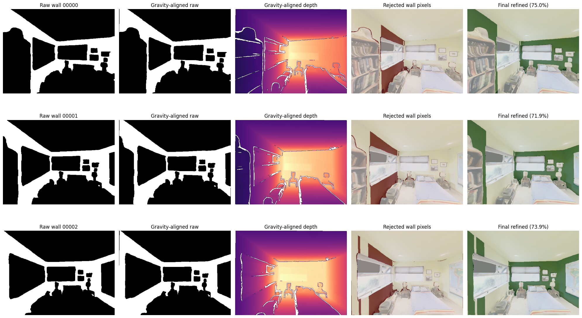
….. 저 창문 날리면 안될것같은데..?
어쨋거나, 가짜벽을 날리고…. 뭔가 벽정보를 추출했다.
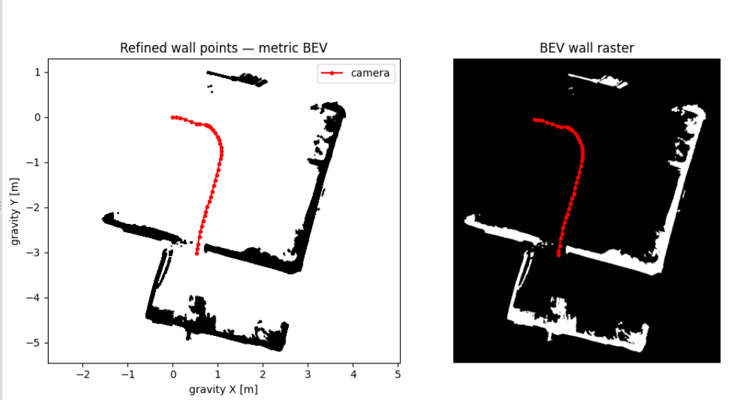
나중에 좀 더 찾아볼 문제이긴 한데, RANSAC 과정에서 free-space violation관련된 항이 있는데 그건 이후에 확인해보자.
4. FloorPlan에서 line/circle 추출/정합
이 논문의 두번째 특이점. 2D CAD 도면과 3D 포인트클라우드에서 BEV로 변환한 이미지간의 정합을 맞추는 과정이 매우 독특하다. 라인과 원을 추출하고 이걸 이용해서 정합을 한다. 정합은 위치만 찾는게 아니라 scale도 찾는 과정을 거치게 된다.
그러기 위해선 어떻게 선과 원을 찾아내는가 먼저 살펴 볼 필요가 있다. 선의 추출은 Seed-Based region growin방식을 사용한다.


Seed based growing이란게 영역/plane을 찾는데는 쉽게 머릿속에 이미지가 떠오르는데, 이걸로 라인을 찾는 방법을 적용하려면 PCA 개념을 가져와야 한다. 이런 방식을 사용한 자료가 있는데, 다음 링크를 참조하면 좋다.
-
Gao et al., “A line segment extraction algorithm using laser data based on seeded region growing” (2018) 링크
-
The Computational Geometry Algorithms Library, CGAL. 링크
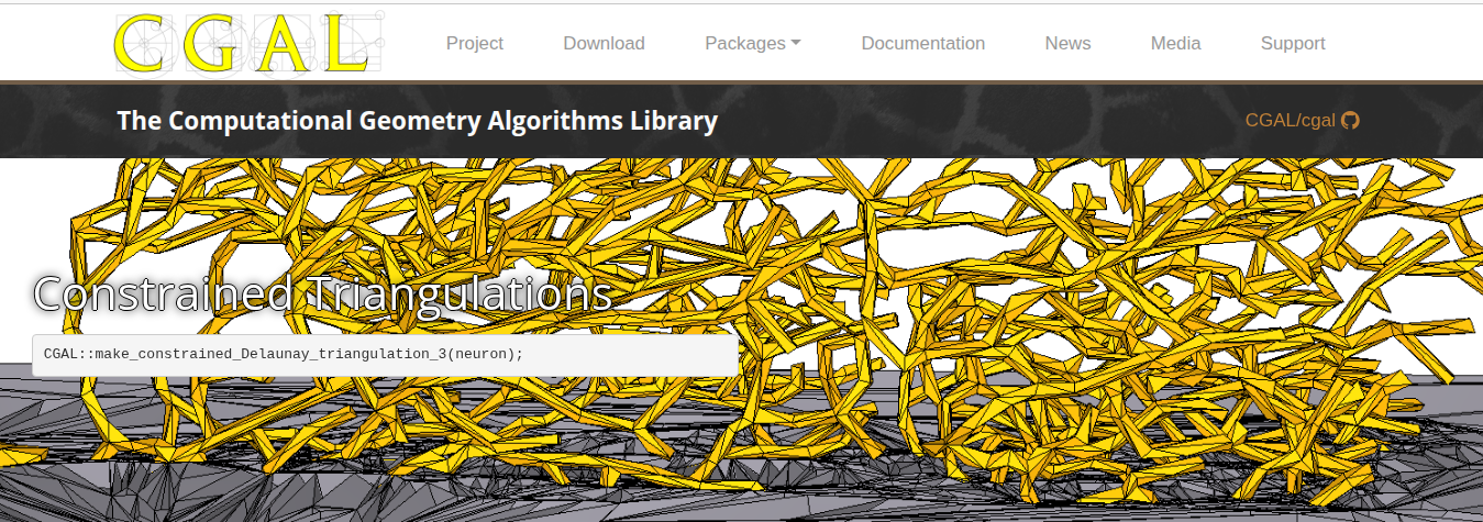
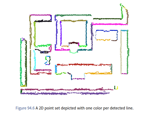
뒤에 찾은 저 라이브러리는 꽤 쓸만할듯 한데. 나중에 좀 더 찾아봐야겠다. 논문에서는 아이디어에 대한 방식만 설명했을 뿐, 정확히 어떤 라이브러리 스타일이라던가, 어떤 알고리즘을 쓴다는 말은 없어서, 이런 부분은 GPT의 영역에 두고자 한다.
혹여 기회가 된다면 다른 Line 추출법도 있는데 비교예시도 만들어보면 좋을 것 같다.
| 방식 | 강점 | 약점 | 잘 맞는 데이터 |
|---|---|---|---|
| Seed-based Region Growing | 연결된 선분을 자연스럽게 분리, local geometry 활용, 선분의 범위를 직접 얻기 쉬움 | seed/threshold에 민감, 노이즈나 gap 때문에 성장 중단 가능 | 정돈된 contour, ordered points, CAD/scan 데이터 |
| Hough Transform | 끊어진 선, 노이즈에 비교적 강함, 전체에서 선 방향 찾기 좋음 | 비슷한 평행선 구분이 애매할 수 있고 discretization 오차 존재 | 이미지 edge map |
| RANSAC | outlier에 매우 강함, 점들이 unordered여도 가능 | 여러 선을 찾으려면 반복 제거 필요, 짧은 선분 분리에 약함 | noisy point cloud |
| Douglas–Peucker | 매우 빠르고 단순, polyline → segment 변환에 좋음 | line detection이라기보다 simplification, noise에 민감 | 이미 연결 순서가 있는 contour |
| Least Squares/PCA | 빠르고 정확한 fitting | outlier에 매우 취약 | 한 선에 속한 점이 이미 정해진 경우 |
Line 추출 코드
코드가 길긴한데.. 아직 완벽히 이해는 못했다. (codex가 구현한 부분인지라…)
- fit_line_least_squares() 여러 점들을 가장 잘 설명하는 직선을 구하는 함수다.
- extract_line_primitives() 아직 어떤 선에도 속하지 않는 seed pixel을 추출하여, 주변점과 함께 직선을 추출해낸다.
def fit_line_least_squares(points: np.ndarray) -> dict[str, np.ndarray | float]:
    points = np.asarray(points, dtype=np.float64)
    if points.ndim != 2 or points.shape[1] != 2 or len(points) < 2:
        raise ValueError(f'line fit은 [N, 2], N>=2가 필요합니다: {points.shape}')
    # 중심을 뺀 covariance의 가장 큰 고유값 방향은 point cloud가 가장 길게 늘어난 접선 방향이다.
    # 그 직교 방향을 unit normal로 삼으면 total least-squares 직선이 된다.
    centroid = points.mean(axis=0)
    centered = points - centroid
    covariance = centered.T @ centered / len(points)
    eigenvalues, eigenvectors = np.linalg.eigh(covariance)
    principal = eigenvectors[:, -1]
    normal = np.array([-principal[1], principal[0]], dtype=np.float64)
    normal /= np.linalg.norm(normal)
    # n/d sign ambiguity를 제거해 serialization과 비교를 deterministic하게 만든다.
    if normal[0] < -1e-12 or (abs(normal[0]) <= 1e-12 and normal[1] < 0):
        normal = -normal
    # normal을 90도 회전해 선을 따라가는 unit direction을 만든다.
    direction = np.array([normal[1], -normal[0]], dtype=np.float64)
    offset = -float(normal @ centroid)
    # support를 direction에 투영한 최솟값/최댓값이 유한 선분의 endpoint와 길이를 정의한다.
    coordinates = centered @ direction
    endpoints = np.stack([
        centroid + float(coordinates.min()) * direction,
        centroid + float(coordinates.max()) * direction,
    ])
    return {
        'normal': normal,
        'offset': offset,
        'direction': direction,
        'endpoints': endpoints,
        'length': float(coordinates.max() - coordinates.min()),
        'centroid': centroid,
        'eigenvalues': eigenvalues,
    }
def extract_line_primitives(
                                points_metric: np.ndarray,
                                pixels_uv: np.ndarray,
                                raster_shape: tuple[int, int],
                                resolution_m: float,
                                parameters: dict,
                                random_seed: int,
                            ) -> tuple[list[dict], dict]:
    points = np.asarray(points_metric, dtype=np.float64)
    pixels = np.asarray(pixels_uv, dtype=np.int32)


    # pixel_to_index는 raster 이웃 (u, v)을 metric point의 row index로 되돌리는 lookup table이다.
    pixel_to_index = np.full(raster_shape, -1, dtype=np.int32)
    pixel_to_index[pixels[:, 1], pixels[:, 0]] = np.arange(len(pixels), dtype=np.int32)
    offsets_uv = pixel_neighbor_offsets(
        float(parameters['connectivity_radius_m']), resolution_m
    )
    # KD-tree는 anchor 주변의 초기 PCA 후보만 빠르게 찾는다. 실제 region 확장은 raster 연결성도 만족해야 한다.
    tree = cKDTree(points)
    generator = np.random.default_rng(random_seed)
    unassigned = np.ones(len(points), dtype=bool)
    accepted_labels = np.full(len(points), -1, dtype=np.int32)
    primitives = []
    rejected_region_count = 0
    rejected_point_count = 0
    total_growth_iterations = 0

    # accepted/rejected 여부와 관계없이 방문한 support를 unassigned에서 제거하므로 각 입력 pixel은 한 raw region에만 속한다.
    while np.any(unassigned):
        available = np.flatnonzero(unassigned)
        anchor = int(available[generator.integers(len(available))])
        local = np.asarray(
            tree.query_ball_point(points[anchor], float(parameters['neighborhood_radius_m'])),
            dtype=np.int64,
        )
        local = local[unassigned[local]]
        if len(local) < 3:
            unassigned[anchor] = False
            rejected_region_count += 1
            rejected_point_count += 1
            continue

        # local PCA는 seed 주변의 초기 가설이고, 아래 반복문에서는 늘어난 support 전체로 다시 적합한다.
        initial_model = fit_line_least_squares(points[local])
        local_distance = np.abs(points[local] @ initial_model['normal'] + initial_model['offset'])
        support = np.unique(local[local_distance <= float(parameters['distance_threshold_m'])])
        if anchor not in support:
            support = np.append(support, anchor)
        # 엄격한 distance threshold에서는 anchor만 남을 수 있다.
        # 한 점으로는 직선을 피팅할 수 없으므로 이 점은 rejected로 처리한다.
        if len(support) < 2:
            unassigned[anchor] = False
            rejected_region_count += 1
            rejected_point_count += 1
            continue
        member = np.zeros(len(points), dtype=bool)
        member[support] = True

        # 현재 support의 raster 이웃 중 line 직교거리 조건도 통과한 점만 추가한다.
        # 더 이상 추가될 점이 없으면 fixed point에 도달한 것이다.
        while True:
            support_indices = np.flatnonzero(member)
            model = fit_line_least_squares(points[support_indices])
            neighbor_uv = (
                pixels[support_indices, None, :] + offsets_uv[None, :, :]
            ).reshape(-1, 2)
            inside = (
                (neighbor_uv[:, 0] >= 0)
                & (neighbor_uv[:, 0] < raster_shape[1])
                & (neighbor_uv[:, 1] >= 0)
                & (neighbor_uv[:, 1] < raster_shape[0])
            )
            neighbor_uv = neighbor_uv[inside]
            candidates = pixel_to_index[neighbor_uv[:, 1], neighbor_uv[:, 0]]
            candidates = np.unique(candidates[candidates >= 0])
            candidates = candidates[unassigned[candidates] & ~member[candidates]]
            if len(candidates) == 0:
                break
            candidate_distance = np.abs(
                points[candidates] @ model['normal'] + model['offset']
            )
            added = candidates[candidate_distance <= float(parameters['distance_threshold_m'])]
            if len(added) == 0:
                break
            member[added] = True
            total_growth_iterations += 1

        # 이 region은 이제 재방문하지 않는다. 작은/짧은 region도 여기서 영구 reject된다.
        support_indices = np.flatnonzero(member)
        unassigned[support_indices] = False
        final_model = fit_line_least_squares(points[support_indices])
        if (
            len(support_indices) >= int(parameters['min_support'])
            and final_model['length'] >= float(parameters['min_length_m'])
        ):
            line_index = len(primitives)
            accepted_labels[support_indices] = line_index
            final_model['support_indices'] = support_indices.astype(np.int32)
            final_model['support_count'] = int(len(support_indices))
            primitives.append(final_model)
        else:
            rejected_region_count += 1
            rejected_point_count += int(len(support_indices))

    # 마지막 assert는 모든 입력 point가 정확히 한 번 accepted 또는 rejected 되었음을 확인한다.
    statistics = {
        'input_point_count': int(len(points)),
        'accepted_line_count': int(len(primitives)),
        'accepted_point_count': int(np.count_nonzero(accepted_labels >= 0)),
        'rejected_region_count': int(rejected_region_count),
        'rejected_point_count': int(rejected_point_count),
        'growth_iterations': int(total_growth_iterations),
        'point_labels': accepted_labels,
    }
    assert statistics['accepted_point_count'] + statistics['rejected_point_count'] == len(points)
    return primitives, statistics
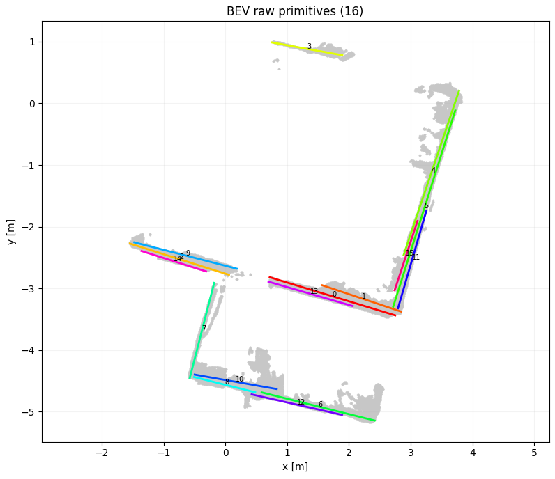
원 추출
원을 찾는 방식은 HDBSCAN 알고리즘을 사용한다. 건물 내부에 원기둥형태나, 둥근 형태의 벽이 있다는 걸 생각해보면 영리한 접근이라고 평가할만하다.
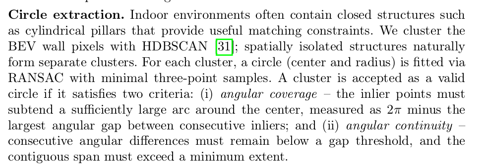
여기선 Gibson 데이터셋만 사용하면서, 원추출에 대한 부분을 생략했는데, 만약 전형적인 예제코드를 사용한다면 다음과 같은 스타일로 작성된다.
import numpy as np
import hdbscan
from skimage.measure import CircleModel, ransac


def detect_circles(points, min_cluster_size=20, residual_threshold=0.1):
    labels = hdbscan.HDBSCAN(
        min_cluster_size=min_cluster_size
    ).fit_predict(points)

    circles = []

    for label in np.unique(labels):
        if label == -1:
            continue

        cluster = points[labels == label]

        model, inliers = ransac(
            cluster,
            CircleModel,
            min_samples=3,
            residual_threshold=residual_threshold,
            max_trials=100
        )

        if model is not None:
            cx, cy, r = model.params
            circles.append([cx, cy, r])

    return np.asarray(circles)
Primitive 추출 결과
3D 맵을 BEV로 변환하여 직선과 원을 추출했으면, 그 과정을 동일하게 2D CAD 맵에서도 수행해야 한다.
이를 위해 선을 좀더 명확하게 하는 과정을 거치는데, morphology closing과 같은 기법들을 이용하여 끊어진 벽을 잇고, 작은 요소들은 제거하는 과정을 거친다.
morphology는 다른 코드 찾다가 실슴한 내용이 있는데, 거기서 사용한 코드는 다음과 같다.
gray_before = cv2.cvtColor(image_before_filtering, cv2.COLOR_BGR2GRAY)
edges_before = cv2.Canny(gray_before, 50, 200)

kernel = np.ones((3, 3), dtype=np.uint8)
morph_iterations = 5  # 10회는 작은 글씨·벽 선을 크게 연결할 수 있습니다.

# 첫 번째 이미지: 원본 흑백 사진을 팽창한 뒤 침식합니다.
gray_dilated = cv2.dilate(gray_before, kernel, iterations=morph_iterations)
gray_morph = cv2.erode(gray_dilated, kernel, iterations=morph_iterations)

# 처리한 흑백 사진에서 Canny 경계를 다시 찾습니다.
edges_after_gray = cv2.Canny(gray_morph, 50, 200)

# 두 번째 이미지: 새 경계 이미지도 팽창한 뒤 침식합니다.
edges_dilated = cv2.dilate(edges_after_gray, kernel, iterations=morph_iterations)
edges_morph = cv2.erode(edges_dilated, kernel, iterations=morph_iterations)

# 09절 이후에는 원본 이미지와 같은 크기의 처리된 경계를 사용합니다.
gray = gray_morph
edges = edges_morph
이 코드를 돌리고서 시각화부분을 붙이면 다음과 같이 보인다. 이런식으로 morphology closing한 다음 라인 추출을 시도한다.
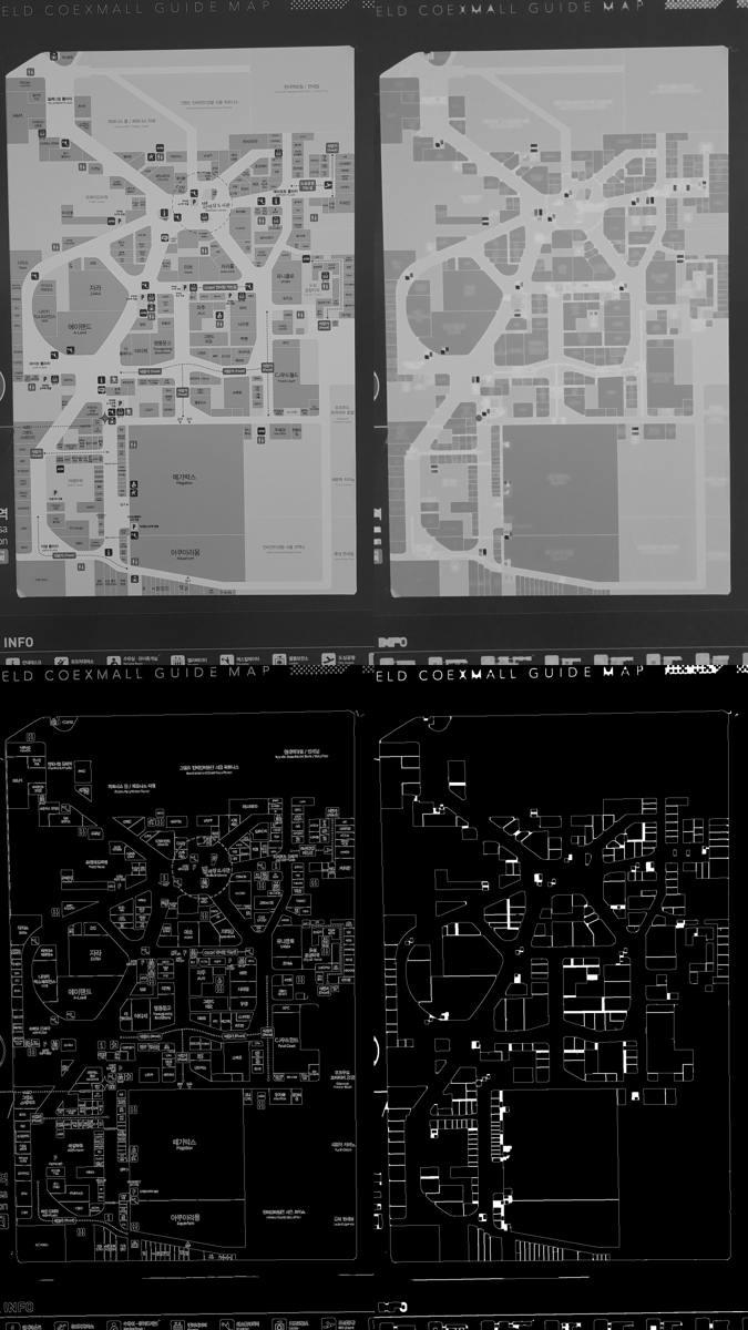
위의 그림과, 데이터셋에서 제공되는 도면을 비교해보면, 그래도 비슷한 결과가 나온다.
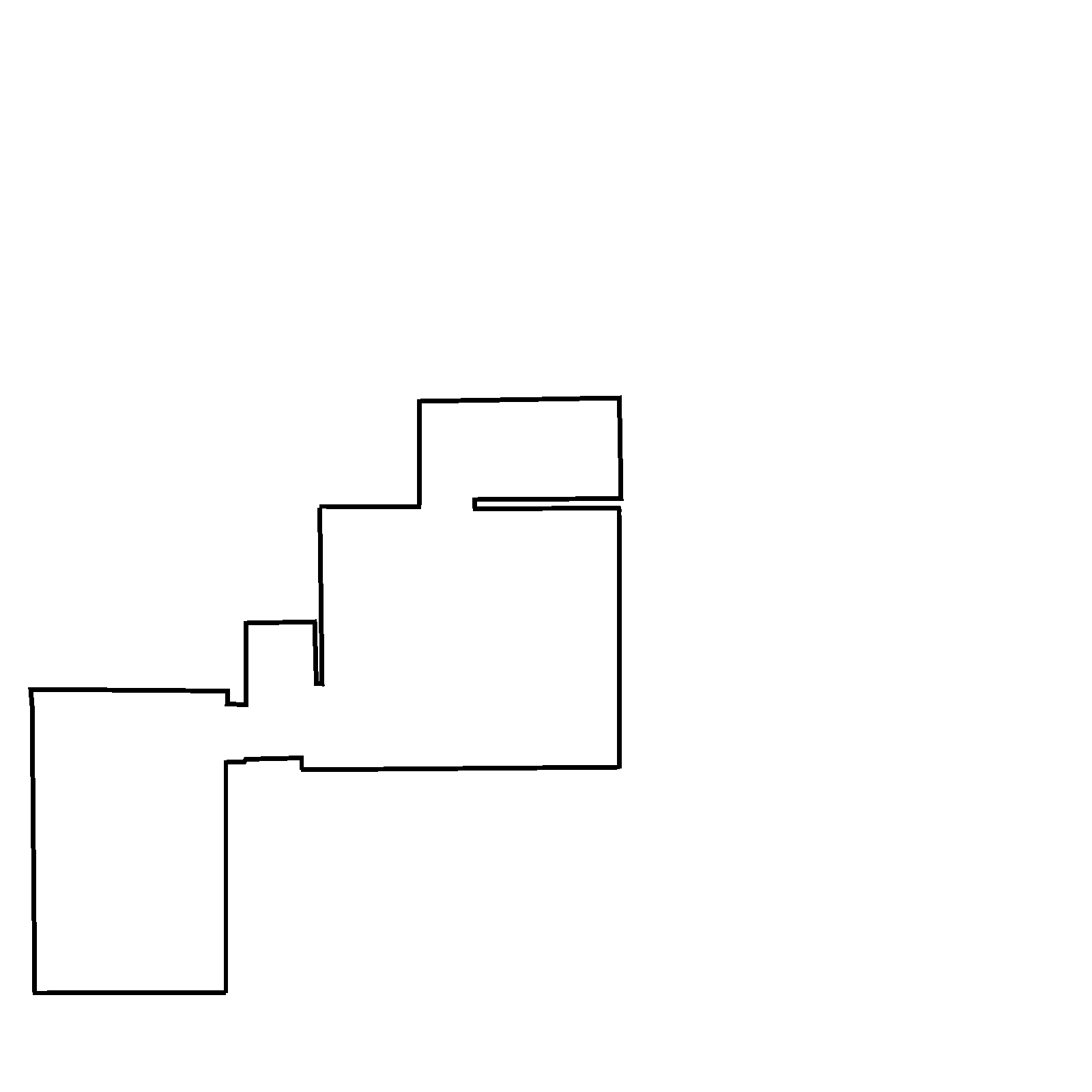
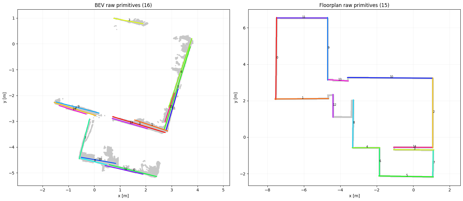
다시금 원래 논문의 예제로 돌아와서, 현재 우리가 사용하고 있과는 데이터셋에서 직선을 추출해보면 다음 그림처럼 보인다. 도면의 원래 품질이 깔끔해서 라인의 추출이 잘되는 편이다.
5. 정합과정. Hybrid RANSAC
논문에선 Model Estimation이라고 표현하고 있다. Feature를 비교하는 solver를 정의하고, 그 solver를 이용해 가설(Pose hypothesis)을 설정하고, 이를 RANSAC 방식으로 평가하며 업데이트 해나간다. 최종적으로 scale,rotation,transform 값은 (s,R,t)를 얻는 것이 목적이다.
1) BEV와 floorplan에서 각각 line/circle primitive를 준비 2) 그중 아주 적은 개수의 primitive correspondence를 샘플링 3) solver를 이용해 similarity transform $(s, R, t)$ 계산, hypothesis 로 저장 4) 2~3의 과정을 반복하여 RANSAC loop 안에서 반복해서 사용하며 많은 hypothesis 생성정 5) Model Scoring 단계에서 어떤 hypothesis가 전체 구조와 가장 잘 맞는지 평가, 선택/탈락 진행
이제 이 과정을 설명하기 위해선 Solver를 먼저 설명해야 한다.
5.1 Solvers
Solver에는 4가지가 있다. 이걸 저자는 minimal solver라 고 말하고 있다.
- 3L : line 3개를 가지고 매칭하는 것
- 2L : line 2개 + scale prior를 가지고 매칭하는 것
- 2C : circle 2개
- LC : line과 circle 1개ㅐ
조금 쉬운 2C부터 보자.
5.1.1 2-Circle solver
BEV에서 2개의 원, 캐드 도면에서 원 두개를 이용해 s,R,t를 구한다.
scale은 두 원의 중심간 거리를 이용해 구한다.원 크기로 하지..왜? 라는 생각을 해보지만, 도면상의 원과 BEV의 원의 크기가 일치한다는 보장은 없으니, 차라리 중심간 거리가 맞을지도 모르겠다.

$\theta$를 구하는 식이 있는데, 이걸 굳이…atan2를 해야 하나 싶다. 내적/cos 으로도 구할 수 있을텐데..
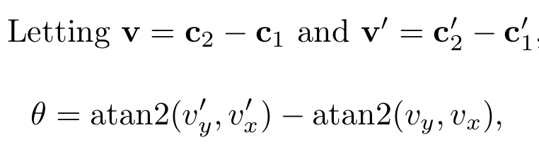
자연스럽게, 이 두선간의 비틀어진 각도를 이용해, rotation 행렬을 구할 수 있고, 원의 중심점간 거리를 통해 translation을 구할 수 있다.

깔끔하다.
5.1.2. 2-Line Solver
우선 첫번째 가정은 scale에서 시작한다. 대략적인 scale값을 추정하고, 이것을 $\tilde{s}$ 라 먼저 정의한다. 그리고 여기에 가우시인 노이즈를 더해 scale의 uncertainty를 허용한다.
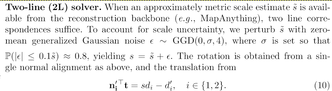
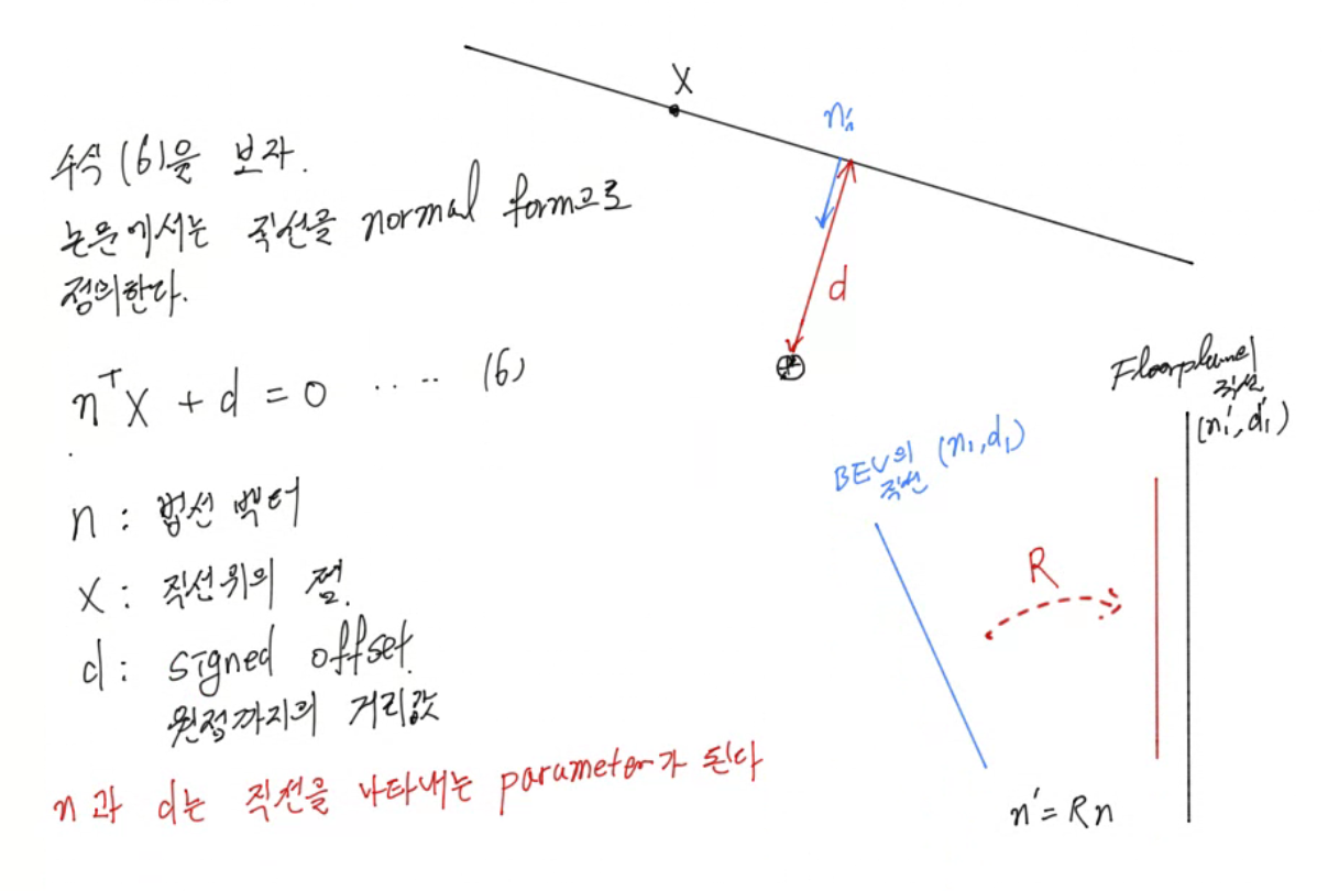
이제 직선에 대해 다뤄보자. 직선에 있는 한 점을 이용하여 방정식을 만들면 다음과 같이 표현할 수 있다. 논문의 수식 (6)에 해당한다.

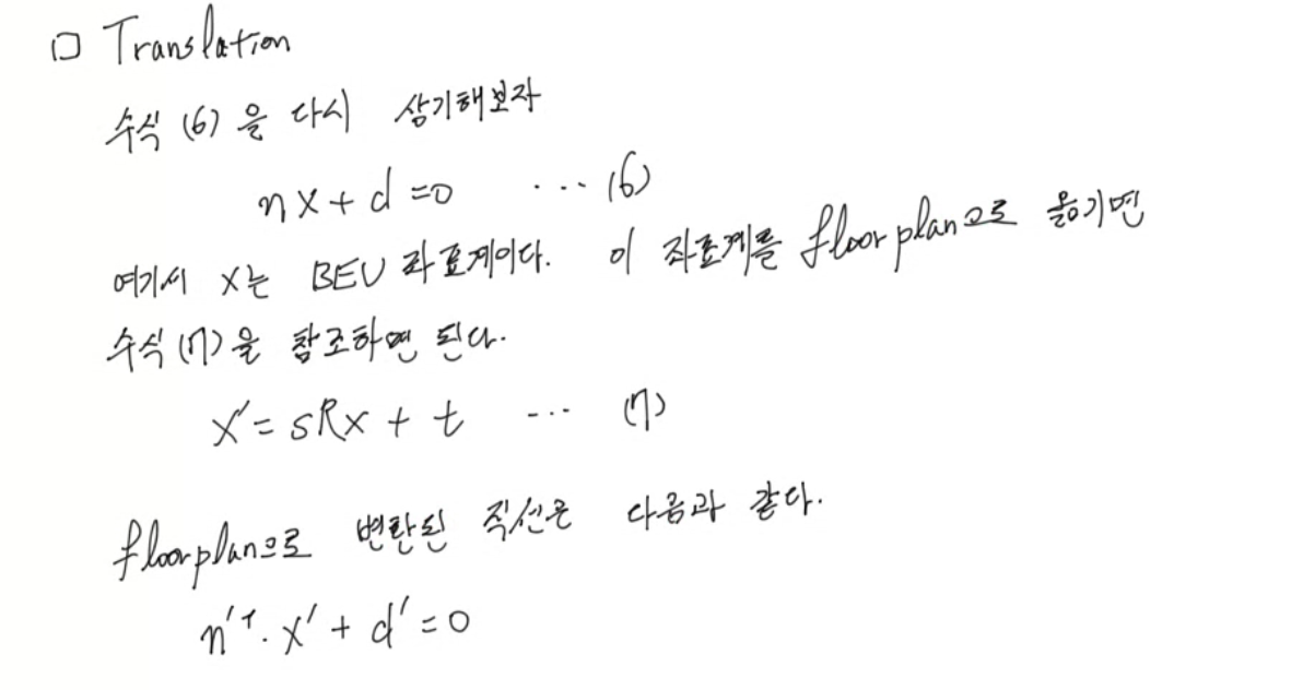
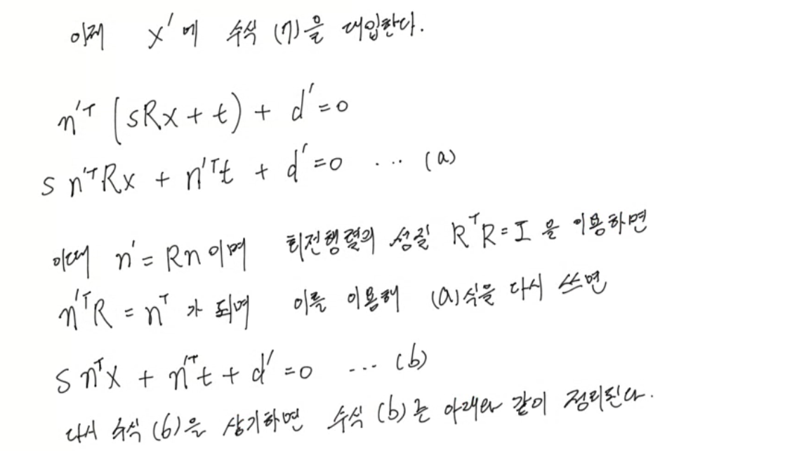
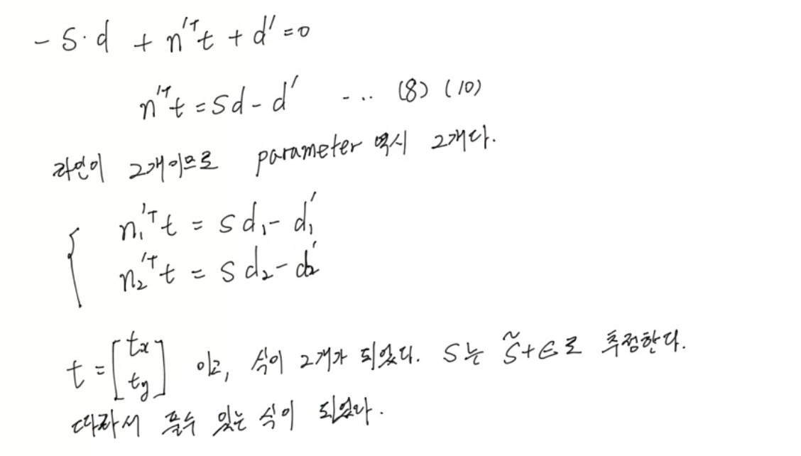
…. 다음번엔 줄공책에 정리해야겠다. 글이 빼뚜룸하네.
5.1.3. 3-Line Solver
2 Line Solver에서는 직선 2개를 쓰기때문에 수식이 2개가 나왔고, 이때문에 scale값 s 를 추정한 상태에서 풀었다면, 이번엔 s도 변술로 바뀐다. 라인이 3개이고, 변수는 s, $t_x,$, $t_y$ 이므로 풀 수 있는 구조가 나온다. 2L 솔버를 이해했다면 어렵지 않다.

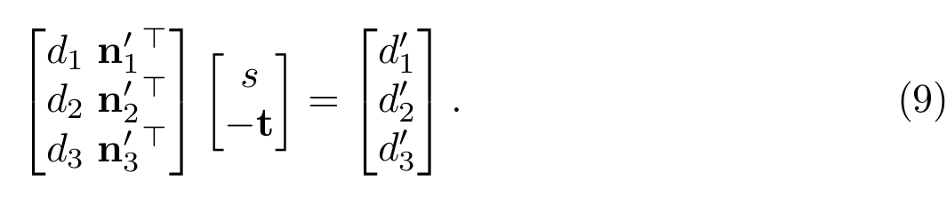
5.1.4. Line-Circle Solver
이젠 선 하나와 원 하나로 s, R, t를 찾아야 한다.
가장 쉽게 R값은 선의 법선으로 알 수 있다. $n’ = Rn$ 이 되므로, R은 쉽게 구해진다.
t와 s를 구해야 하는데, 여기선 scale s를 먼저 구해본다.
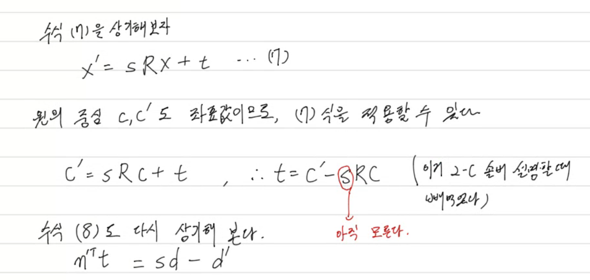
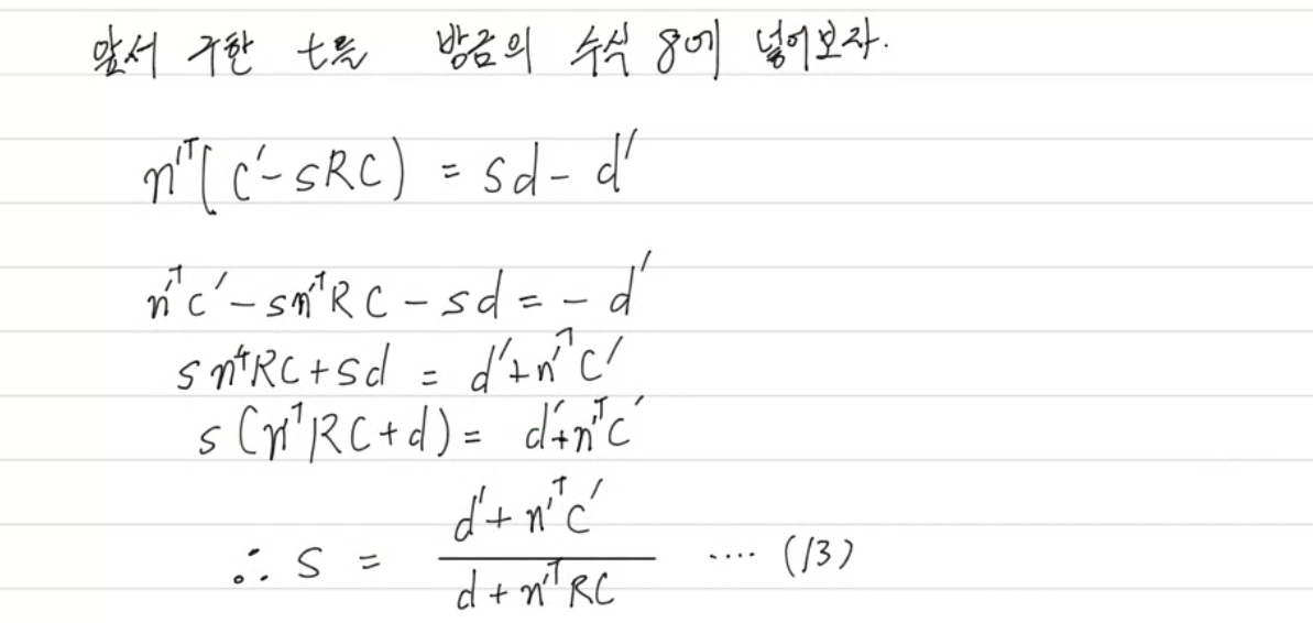
이제 R,s를 구했으니, translation t를 구할수 있게 되었다.

솔버에 대한 설명은 끝났다.
5.2 Hybrid RANSAC
이제 이 네개의 solver를 가지고 RANSAC 루프에 들어간다. 핵심은 RANSAC 한번에 네개의 solver 모두를 다 돌리는게 아니라 매 iteration마다 3L / 2L / 2C / LC 중 하나를 랜덤하게 선택해서 가설(hypotheesis) 만든다는ㄴ 것이다. 이걸 하이브리드 RANSAC이라고 표현하고 있다. (참조: Camposeco, F., Cohen, A., Pollefeys, M., Sattler, T.: Hybrid camera pose estima-tion. In: CVPR (2018)) Pollefeys 이분… 자주 등장하네.
Hybrid RANSAC과 관련된 부분은 다음과 같은 순서로 진행된다.
function run_hybrid_ransac(seed):

    RNG(난수생성기) 초기화
    hypotheses = []

    반복(num_iterations):

        solver ← 3L 또는 2L 무작위 선택

        if solver == 3L:
            대응 line 3개 샘플링
            candidates ← 3L solver 실행

        else:
            대응 line 2개 샘플링
            scale ← scale prior에서 샘플링
            candidates ← 2L solver 실행

        for candidate in candidates:
            candidate의 coarse consistency score 계산
            hypotheses에 저장

    return hypotheses
Hybrid RANSAC 만 가지고는 문제가 하나 더 있다. correspondece를 찾는 과정에서 전부 나열해 찾는다면, floorplan의 라인 개수가 많아졌을때 경우의 수가 폭증하게 된다.
이걸 줄이기 위해 논문에선 세가지 pruning 전략을 사용한다. 그리고 이 pruning 전략은 3L 솔버에서만 적용한다.
1) Line deduplication 방향과 offset이 매우 비슷한 거의 중복된 line은 제거한다. 이때는 더 긴 segment를 남긴다. BEV와 floorplan양쪽에서 수행한다.
2) Spartial proximity BEV는 local 영역만을 나타낸다. 따라서, floorplan에서 3개의 line을 샘플링할때, 서로 공간적으로 가까운 후보들만 선택한다. 이를 위해 line 사이의 거리를 미리 계산해둔다. 이를 통해 line triplet 의 구성시 조합수가 제곱에 비례하는 것을 quasi-linear수준으로 낮출 수 있다.
3) Normal consistency 하나의 line correspondence로부터 rotation $\mathbf R$을 추정한 뒤, 나머지 두 line까지 포함한 세 line의 normal이 BEV의 대응 line normal과 모두 일관되어야 한다. $\tau_p$는 cosine similarity threshold 인데, 다시말해, 평행하게 잘 일치하는지를 확인하는 과정이다. 이 조건을 만족시키지 못하면 scale과 translation을 계산하기 전에 가설에서 제외한다.

결국, 선의 개수를 좀 줄여놓고, 선들간에 미리 조합 계산해두고. 그리고 돌려봐서 어느정도 일치하지 않으면 빼버린다는 소리군.
5.3 코드
Gibson 데이터셋은 원이 없다. (두둥 탁)
따라서, 3L과 2L 솔버만 구현하고 이걸 RANSAC으로 돌리는 코드를 확인해보자.
우선, 앞서 수식유도에서 사용되었던 기본 연산식들이다. 좌표변환을 수행하는 Sim(2)와 Line 관련 유틸리티들이다.
def wrap_angle(angle: float) -> float:
    return float((angle + np.pi) % (2.0 * np.pi) - np.pi)


def rotation_matrix(theta: float) -> np.ndarray:
    cosine, sine = np.cos(theta), np.sin(theta)
    return np.array([[cosine, -sine], [sine, cosine]], dtype=np.float64)


def normal_alignment_angle(source_normal: np.ndarray, target_normal: np.ndarray) -> float:
    # 대응하는 법선의 방향 차이로 후보 회전을 만든다. 직선의 법선은 부호가
    # 뒤집힐 수 있으므로 solver에서는 이 각도와 pi를 더한 각도를 모두 검사한다.
    return wrap_angle(
        np.arctan2(target_normal[1], target_normal[0])
        - np.arctan2(source_normal[1], source_normal[0])
    )


def validate_line_parameters(normals: np.ndarray, offsets: np.ndarray, expected_count: int):
    # 모든 solver가 unit-normal Hesse form n^T x + d = 0을 공유한다.
    # 단위 법선이 아니면 offset의 metric 의미와 scale 식이 달라지므로 초기에 거절한다.
    normals = np.asarray(normals, dtype=np.float64)
    offsets = np.asarray(offsets, dtype=np.float64)
    if normals.shape != (expected_count, 2) or offsets.shape != (expected_count,):
        raise ValueError(
            f'expected normals {(expected_count, 2)}, offsets {(expected_count,)}; '
            f'got {normals.shape}, {offsets.shape}'
        )
    if not np.all(np.isfinite(normals)) or not np.all(np.isfinite(offsets)):
        raise ValueError('line parameters must be finite')
    norms = np.linalg.norm(normals, axis=1)
    if not np.allclose(norms, 1.0, atol=1e-6):
        raise ValueError('line normals must be unit vectors')
    return normals, offsets


def transform_lines(
    normals: np.ndarray,
    offsets: np.ndarray,
    scale: float,
    rotation: np.ndarray,
    translation: np.ndarray,
) -> tuple[np.ndarray, np.ndarray]:
    # x_t = s R x_s + t 를 n^T x + d = 0에 대입하면
    # n_t = R n_s, d_t = s d_s - n_t^T t가 된다. 아래는 synthetic 검증과
    # solver의 선형식을 동일한 좌표/부호 convention으로 연결하는 기준 구현이다.
    target_normals = np.asarray(normals, dtype=np.float64) @ rotation.T
    target_offsets = scale * np.asarray(offsets, dtype=np.float64) - target_normals @ translation
    return target_normals, target_offsets


def transform_points(
    points: np.ndarray, scale: float, rotation: np.ndarray, translation: np.ndarray
) -> np.ndarray:
    return scale * (np.asarray(points, dtype=np.float64) @ rotation.T) + translation


def rotation_error(first: np.ndarray, second: np.ndarray) -> float:
    relative = first @ second.T
    return abs(wrap_angle(np.arctan2(relative[1, 0], relative[0, 0])))
3L 변환과 관련된 부분은 다음과 같다.
def solve_3l(
    source_normals: np.ndarray,
    source_offsets: np.ndarray,
    target_normals: np.ndarray,
    target_offsets: np.ndarray,
    parameters: dict,
) -> list[dict]:
    """세 line correspondence로 scale, rotation, translation을 복원한다.

    회전 후보를 정하면 각 대응선은 s * d_source - n_target^T t = d_target가 된다.
    세 식을 [d_source, n_target_x, n_target_y] [s, -t_x, -t_y]^T = d_target
    로 쌓아 3x3 선형계로 푼다.
    """
    # 입력은 sampler가 만든 순서 있는 correspondence이며, shape/unit-normal을
    # 검증해 잘못된 cache나 caller 오류가 수치 해로 섞이는 것을 막는다.
    source_normals, source_offsets = validate_line_parameters(source_normals, source_offsets, 3)
    target_normals, target_offsets = validate_line_parameters(target_normals, target_offsets, 3)
    # 첫 대응선으로 회전의 기준 각을 정한다. n과 -n이 같은 기하 직선을
    # 표현하므로 180도 ambiguity를 아래 loop에서 명시적으로 전개한다.
    base_theta = normal_alignment_angle(source_normals[0], target_normals[0])
    hypotheses = []

    for theta in (base_theta, wrap_angle(base_theta + np.pi)):
        # 두 법선 방향 가설 각각에 대해 나머지 두 대응선도 같은 회전과
        # 양립하는지 확인한 뒤, 양립할 때만 scale/translation을 계산한다.
        rotation = rotation_matrix(theta)
        rotated_normals = source_normals @ rotation.T
        normal_dots = np.sum(rotated_normals * target_normals, axis=1)
        # |dot|가 1에 가까워야 회전 후 법선이 target 법선 또는 그 반대와
        # 일치한다. 낮으면 correspondence 자체가 이 rotation과 모순된다.
        if np.min(np.abs(normal_dots)) < float(parameters['normal_consistency_cosine']):
            continue

        # line (n, d)와 (-n, -d)는 동일하다. dot의 부호로 target line의
        # 표현을 정렬해 offset 식에서 부호 ambiguity를 없앤다.
        signs = np.where(normal_dots >= 0.0, 1.0, -1.0)
        aligned_target_normals = signs[:, None] * target_normals
        aligned_target_offsets = signs * target_offsets
        # Eq. (9)의 3x3 계수행렬. rank 부족은 평행/중복 line 등으로 인해
        # scale 또는 translation이 유일하게 정해지지 않는 퇴화 최소 샘플이다.
        system = np.column_stack([source_offsets, aligned_target_normals])
        if np.linalg.matrix_rank(system) < 3:
            continue
        # full rank라도 조건수가 너무 크면 작은 offset/normal 오차가 pose를
        # 크게 흔드므로, RANSAC 후보로 사용하지 않고 샘플을 거절한다.
        condition_number = float(np.linalg.cond(system))
        if not np.isfinite(condition_number) or condition_number > float(parameters['max_condition_number']):
            continue

        # solution = [scale, -translation_x, -translation_y].
        # solve를 사용해 역행렬을 명시적으로 만들지 않아 수치 오차를 줄인다.
        solution = np.linalg.solve(system, aligned_target_offsets)
        scale = float(solution[0])
        translation = -solution[1:]
        if not np.isfinite(scale) or scale <= float(parameters['min_scale']):
            continue
        # 음수/0 scale은 좌표계를 반전하거나 붕괴시키므로 물리적으로 유효한
        # Sim(2) 가설이 아니다. residual은 뒤에서 solver 품질을 진단하는 값이다.
        residual = system @ solution - aligned_target_offsets
        hypotheses.append({
            'solver': '3L',
            'scale': scale,
            'rotation': rotation,
            'theta': theta,
            'translation': translation,
            'normal_signs': signs.astype(np.int8),
            'normal_consistency': np.abs(normal_dots),
            'condition_number': condition_number,
            'max_equation_residual': float(np.max(np.abs(residual))),
        })
    return hypotheses
2 Line Solver의 구현은 다음과 같다.
def normals_are_parallel(normals: np.ndarray, angle_threshold_deg: float) -> bool:
    # |cross(n1, n2)| = |sin(angle)|. 2L은 translation의 2개 성분을
    # 두 target normal로 풀기 때문에 두 법선이 평행이면 역행렬이 존재하지 않는다.
    sine = abs(float(
        normals[0, 0] * normals[1, 1] - normals[0, 1] * normals[1, 0]
    ))
    return sine <= np.sin(np.deg2rad(angle_threshold_deg))


def solve_2l(
    source_normals: np.ndarray,
    source_offsets: np.ndarray,
    target_normals: np.ndarray,
    target_offsets: np.ndarray,
    scale: float,
    parameters: dict,
) -> list[dict]:
    """두 line correspondence와 외부 scale 표본으로 Sim(2)를 복원한다.

    Scale은 이 최소 문제에서 관측되지 않으므로 RANSAC이 제공한 prior sample을
    고정한다. 회전/부호를 정렬한 뒤 2x2 식 n_target^T t = s*d_source - d_target를
    풀어 translation을 얻는다.
    """
    source_normals, source_offsets = validate_line_parameters(source_normals, source_offsets, 2)
    target_normals, target_offsets = validate_line_parameters(target_normals, target_offsets, 2)
    # 2L의 scale은 solver 내부에서 재추정하지 않는다. prior 표본이 유효하지
    # 않으면 이후 선형계도 의미가 없으므로 즉시 빈 후보 집합을 돌려준다.
    if not np.isfinite(scale) or scale <= float(parameters['min_scale']):
        return []
    angle_threshold = float(parameters['parallel_angle_threshold_deg'])
    # source 또는 target pair가 평행하면 제약 두 개가 독립적이지 않다.
    # 특히 target pair 평행은 translation 선형계가 singular함을 뜻한다.
    if normals_are_parallel(source_normals, angle_threshold) or normals_are_parallel(target_normals, angle_threshold):
        return []

    base_theta = normal_alignment_angle(source_normals[0], target_normals[0])
    hypotheses = []
    for theta in (base_theta, wrap_angle(base_theta + np.pi)):
        # 3L과 동일하게 line-normal 부호 ambiguity에 대한 두 회전 가지를
        # 모두 검사한다. 이 단계는 scale prior와 독립적인 기하 검증이다.
        rotation = rotation_matrix(theta)
        rotated_normals = source_normals @ rotation.T
        normal_dots = np.sum(rotated_normals * target_normals, axis=1)
        if np.min(np.abs(normal_dots)) < float(parameters['normal_consistency_cosine']):
            continue
        signs = np.where(normal_dots >= 0.0, 1.0, -1.0)
        aligned_target_normals = signs[:, None] * target_normals
        aligned_target_offsets = signs * target_offsets
        # 2x2 target-normal 행렬의 conditioning을 확인한다. 거의 평행한 선은
        # 앞의 angle threshold를 통과할 수도 있으므로 추가 안전장치가 필요하다.
        condition_number = float(np.linalg.cond(aligned_target_normals))
        if not np.isfinite(condition_number) or condition_number > float(parameters['max_condition_number']):
            continue
        # 고정된 scale에서 남은 미지수는 translation뿐이다. 이 식은 line
        # transform d_t = s*d_s - n_t^T*t를 translation에 대해 정리한 것이다.
        right_hand_side = scale * source_offsets - aligned_target_offsets
        translation = np.linalg.solve(aligned_target_normals, right_hand_side)
        # exact minimal solver에서는 residual이 수치 정밀도 수준이어야 한다.
        # 값은 버리지 않고 hypothesis에 담아 synthetic/RANSAC 진단에 사용한다.
        residual = aligned_target_normals @ translation - right_hand_side
        hypotheses.append({
            'solver': '2L',
            'scale': float(scale),
            'rotation': rotation,
            'theta': theta,
            'translation': translation,
            'normal_signs': signs.astype(np.int8),
            'normal_consistency': np.abs(normal_dots),
            'condition_number': condition_number,
            'max_equation_residual': float(np.max(np.abs(residual))),
        })
    return hypotheses
실제 구현된 코드는 다음과 같다.
def run_hybrid_ransac(random_seed: int) -> tuple[list[dict], dict]:
    """한 seed에서 3L/2L 최소 샘플 가설을 생성하고 coarse 점수만 계산한다.

    RANSAC의 한 iteration은 '최소 대응 집합 하나 -> 가능한 모든 해(candidate)'이다.
    따라서 하나의 최소 solver가 복수의 Sim(2) 해를 반환하면, 모두 보존한 뒤
    다음 단계의 coarse-to-fine ranking에서 기하 일관성으로 구분한다.
    """
    # Seed별 RNG를 분리해 실행 결과를 재현하고, seed 간 독립적인 표본을 만든다.
    generator = np.random.default_rng(random_seed)
    enabled = list(ransac_cfg['enabled_solvers'])
    hypotheses = []
    selected_counts = {name: 0 for name in enabled}
    empty_solver_outputs = 0
    start = time.perf_counter()

    # --- RANSAC sampling loop -------------------------------------------------
    # 매 반복은 무작위 최소 샘플로 하나 이상의 pose 가설을 제안한다. 아직
    # 최적 가설을 고르지 않으며, 이 cell은 후보 생성과 저비용 coarse scoring만 한다.
    for iteration in range(int(ransac_cfg['num_iterations'])):
        # Hybrid RANSAC: 3L(스케일을 함께 풂) 또는 2L(스케일 prior 필요)를
        # 균등 확률로 선택한다. 선택 횟수는 solver 편향을 확인하기 위해 기록한다.
        solver_type = enabled[int(generator.integers(len(enabled)))]
        selected_counts[solver_type] += 1
        if solver_type == '3L':
            # 사전 구축한 유효 3-line 대응 pool에서 한 triplet을 균등 샘플링한다.
            # 3L은 Sim(2)의 scale까지 기하적으로 결정하므로 별도 scale 표본이 없다.
            source_indices, target_indices = correspondence_pool_3l[
                int(generator.integers(len(correspondence_pool_3l)))
            ]
            candidates = solve_3l_indices(source_indices, target_indices)
            sampled_scale = np.nan
        elif solver_type == '2L':
            # 2L 최소 문제는 scale이 부족하므로, 대응 pair와 scale prior를 함께 뽑는다.
            source_indices, target_indices = correspondence_pool_2l[
                int(generator.integers(len(correspondence_pool_2l)))
            ]
            # GGD prior에서 scale을 표본화한다. prior_mean을 중심으로 한 이 값은
            # solver 입력일 뿐이며, 뒤의 dense consistency score가 가설을 평가한다.
            sampled_scale = prior_mean + float(
                gennorm.rvs(
                    prior_beta, scale=prior_scale_parameter, random_state=generator
                )
            )
            candidates = solve_2l_indices(source_indices, target_indices, sampled_scale)
        else:
            raise ValueError(f'unsupported Gibson solver: {solver_type}')
        # 퇴화된 샘플 또는 수치적으로 불가능한 경우 solver가 빈 결과를 반환할 수 있다.
        # 이 표본은 inlier/outlier 판정을 시도하지 않고 다음 무작위 표본으로 넘어간다.
        if not candidates:
            empty_solver_outputs += 1
            continue
        # 최소 solver는 대칭성 때문에 여러 해를 낼 수 있다. 하나도 임의로 버리지 않고
        # 각 해를 별도의 RANSAC 가설로 채점해 후속 ranking에 전달한다.
        for candidate_id, hypothesis in enumerate(candidates):
            hypothesis.update({
                'random_seed': int(random_seed),
                'iteration': int(iteration),
                'candidate_id': int(candidate_id),
                'source_indices': tuple(int(x) for x in source_indices),
                'target_indices': tuple(int(x) for x in target_indices),
                'sampled_scale': float(sampled_scale),
            })
            # Provenance는 결과 재현/디버깅용이다: 어떤 seed, 반복, 최소 샘플과
            # 2L scale 표본에서 이 가설이 나왔는지 저장한다.
            hypothesis['coarse_consistency'] = consistency_score(
                bev_coarse_points, hypothesis, tau_c_m
            )
            # 전체 wall-point가 후보 Sim(2)에 얼마나 일관되는지 coarse threshold
            # tau_c_m로 평가한다. 이 점수로 후보를 shortlist한 뒤 fine score를 계산한다.
            hypotheses.append(hypothesis)

    # Sampling 자체의 품질/비용을 보고할 통계. 빈 solver 결과는 후보 수와
    # iteration 수가 다른 이유를 설명하므로 명시적으로 남긴다.
    statistics = {
        'seed': int(random_seed),
        'iterations': int(ransac_cfg['num_iterations']),
        'solver_selection_counts': selected_counts,
        'empty_solver_outputs': int(empty_solver_outputs),
        'generated_hypotheses': int(len(hypotheses)),
        'runtime_seconds': float(time.perf_counter() - start),
    }
    return hypotheses, statistics


all_hypotheses = []
seed_statistics = []
# 여러 seed를 실행해 특정 난수열에 대한 의존도를 낮춘다. 각 seed의 모든 후보를
# 합친 뒤, 다음 cell에서 seed별 coarse top-k를 먼저 선택한다.
for random_seed in part6_cfg['random_seeds']:
    seed_hypotheses, statistics = run_hybrid_ransac(int(random_seed))
    all_hypotheses.extend(seed_hypotheses)
    seed_statistics.append(statistics)
    print(statistics)
assert all_hypotheses
print('total hypotheses:', len(all_hypotheses))
6. Model Scoring
Model Scoring은 앞 단계의 hybrid RANSAC이 만든 여러 similarity transform hypothesis 중에서 어떤 정합 후보가 가장 그럴듯한지 점수로 평가하는 단계다.
6.1 Consistency score $\mathcal{C}^c$
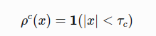
먼저 식(15)를 보자. $x_1$은 BEV 좌표계의 포인트를 Floorplan으로 변환한 좌표값이고, $X_2$는 Floorplan의 벽 포인트 집합이다. $X_2$ 의 점들 중 $x_1$과의 가장 가까운 점과의 거리를 수식으로 표현한 것이 식 (15)인 것이다.

그러면, 이제 이 식을 이용해서, BEV좌표의 모든 점을 옮겨가자. 그게 $\mathcal{T}(x_w;s,R,t)$ 다. 그 점들과 캐드도면의 벽 픽셀들 $X’_w$ 과의 거리가 $\tau$ 이내로 들어올 경우 1점을 준다. 그게 $\rho^c$ 다. 모든 픽셀에 대해 이 값들을 다 더한다음 평균을 내면 Consistency score가 된다. 그게 수식 (16)이다.

6.1 Violation score $\mathcal{C}^v$
앞서 말한 Consistency score와 달리, Violation score는 변환이 방향부터 반대다. floorplan에서 “벽”이라고 되어 있는 위치가 BEV에서 관측된 free space 안으로 들어오지는 않는가? 를 계산한다.
floorplan의 벽 픽셀을 BEV영역으로 가져온다.
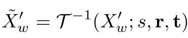
그 다음, 벽픽셀과 뻥 뚫린 공간사이의 겹치는 픽셀들을 찾는다.
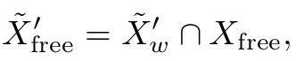
그리고 그 겹친 픽셀들과 벽 사이의 거리가 얼마나 가까운가에 대해 계산하고, 임계치를 넘은 픽셀의 개수를 카운트해 비율로 표현한다. 이게 수식 (17)이다.

Final hypothesis score
앞서 언급한 두개의 score의 차이를 구하면 된다. (벽이 잘 매칭이 되었는가) - (벽이 잘봇 매칭되었는가) 잘 매칭되었다면 1에 가깝게 되고, 잘못매칭되면 -1에 가깝게 움직인다.

그럼 이렇게 만들어진 score는 어디다 쓰는가? 바로 Hybrid RANSAC에서 hypothesis를 평가하는데 사용한다. 왜… 이걸 hypothesis라 하는지 모르겠다. 그냥 localization socore라고 해도 되지 않나 싶긴 한데..
for each RANSAC iteration:

    1. solver를 하나 선택
       solver ∈ {3L, 2L, 2C, LC}

    2. 선택된 solver에 맞는 minimal sample 추출

    3. minimal sample로 similarity transform hypothesis 계산
       H = (s, R, t)

    4. hypothesis 평가
       Cc = consistency_score(H)
       Cv = violation_score(H)

    5. 최종 score 계산
       C = Cc - Cv

    6. 현재 best score보다 높으면
       best_H = H
       best_score = C

return best_H
코드의 구현은 다음과 같다. 이 계산을 RANSAC 중 계속 수행한다.
def transform_points(points: np.ndarray, hypothesis: dict) -> np.ndarray:
    # hypothesis는 BEV metric 좌표를 floorplan metric 좌표로 보내는 Sim(2)이다:
    # p_floor = scale * R * p_bev + translation. consistency score는 이 방향을 쓴다.
    return hypothesis['scale'] * (points @ hypothesis['rotation'].T) + hypothesis['translation']


def inverse_transform_points(points: np.ndarray, hypothesis: dict) -> np.ndarray:
    # 위 Sim(2)의 역변환이다. violation score에서는 floorplan의 벽을 관측 BEV
    # free-space와 비교해야 하므로 floorplan -> BEV 방향이 필요하다.
    return ((points - hypothesis['translation']) @ hypothesis['rotation']) / hypothesis['scale']


def consistency_score(points: np.ndarray, hypothesis: dict, threshold_m: float) -> float:
    """변환된 점 중 floorplan 벽 threshold 이내에 있는 비율(C^c)을 반환한다.

    distance field를 사용하므로 모든 점-벽 segment 거리를 다시 계산하지 않는다.
    결과는 [0, 1] 범위이며, 1은 모든 입력 점이 floorplan wall과 일관됨을 뜻한다.
    """
    # BEV wall point를 후보 pose로 floorplan metric 좌표에 정렬한다.
    transformed = transform_points(points, hypothesis)
    distances, _, _ = sample_distance_field(
        transformed, floorplan_wall_distance_m, T_floor_px_from_metric
    )
    # 각 변환 점에서 가장 가까운 floorplan wall까지의 거리를 조회하고,
    # 허용 오차 이내인 점의 비율을 inlier-like consistency로 사용한다.
    return float(np.mean(distances < threshold_m))


def violation_score(hypothesis: dict, threshold_m: float) -> tuple[float, int]:
    """관측 free-space 안에 놓인 floorplan 벽의 비율(C^v)과 표본 수를 반환한다.

    좋은 pose라면 floorplan의 벽은 BEV에서 벽/미관측 영역에 놓여야 한다. 따라서
    명확히 비어 있다고 관측된 곳에 위치하고 clearance가 큰 벽은 위반으로 센다.
    """
    # 가설을 역적용해 floorplan wall sample을 BEV metric 좌표로 되돌린다.
    inverse_floor_walls = inverse_transform_points(floorplan_wall_points, hypothesis)
    # BEV free-space mask를 인덱싱할 수 있도록 metric 좌표를 pixel (u, v)로 바꾼다.
    uv = metric_to_uv(inverse_floor_walls, T_bev_px_from_metric)
    rounded = np.rint(uv).astype(np.int64)
    # 이미지 밖의 sample은 관측 여부를 판정할 수 없으므로 free-space 위반에서 제외한다.
    inside = (
        (rounded[:, 0] >= 0) & (rounded[:, 0] < bev_free_space.shape[1])
        & (rounded[:, 1] >= 0) & (rounded[:, 1] < bev_free_space.shape[0])
    )
    # inside AND bev_free_space인 sample만 '벽이 비어 있는 관측 공간에 들어감'을
    # 검증할 근거가 있다. 나머지는 unknown으로 취급해 패널티를 주지 않는다.
    in_observed_free = np.zeros(len(inverse_floor_walls), dtype=bool)
    in_observed_free[inside] = bev_free_space[rounded[inside, 1], rounded[inside, 0]]
    count = int(in_observed_free.sum())
    if count == 0:
        # 비교 가능한 free-space 교집합이 없을 때의 score는 논문에 명시되지 않아
        # config의 보수적 기본값(현재 0.0)으로 처리하고 표본 수도 함께 반환한다.
        return float(scoring_cfg['empty_free_intersection_violation']), 0
    # free-space 내부에서도 실제 BEV 벽에서 멀리 떨어질수록 위반이 더 확실하다.
    # clearance distance field에서 그 거리를 읽어 threshold 초과 비율을 계산한다.
    clearance, _, _ = sample_distance_field(
        inverse_floor_walls[in_observed_free],
        bev_clearance_distance_m,
        T_bev_px_from_metric,
    )
    return float(np.mean(clearance > threshold_m)), count


# 설정은 pixel 단위이므로 각 grid의 m/pixel 해상도를 곱해 두 score의 metric
# threshold로 변환한다. floorplan consistency와 BEV violation은 서로 다른 grid를 쓴다.
tau_c_m = float(scoring_cfg['tau_c_px']) * floorplan_resolution
tau_v_m = float(scoring_cfg['tau_v_px']) * bev_resolution
print('tau_c/tau_v [m]:', tau_c_m, tau_v_m)
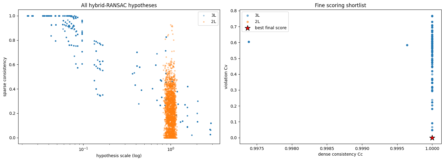
이걸 전체 RANSAC과정에서 기록하면서 점도표로 찍어보면 이런식이다.
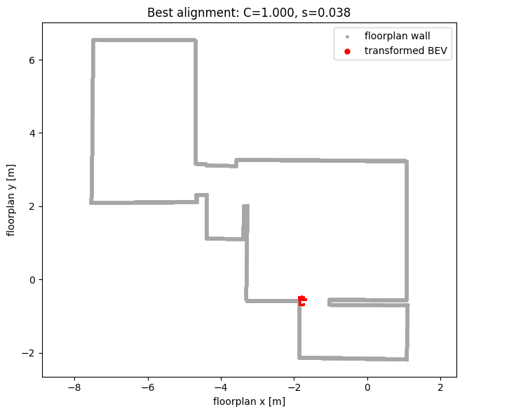
그래서 최종선택한 지점은 여기다.
Model refinement
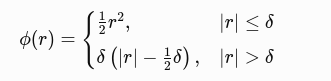
최고 점수 hypothesis를 조금 더 정확하게 미세 조정하는 단계다.

$\phi ()$ 는 Huber loss 를 의미한다. Huber loss는 작은 오차에는 제곱 오차(L2)처럼 반응하고, 큰 오차에는 절대값 오차(L1)처럼 반응하는 손실 함수다. 최적화 함수는 LM optimization을 사용한다.
실험 결과.
위에서 나온 일련의 과정을 거쳐 카메라 포즈를 추정해보면 다음과 같다.
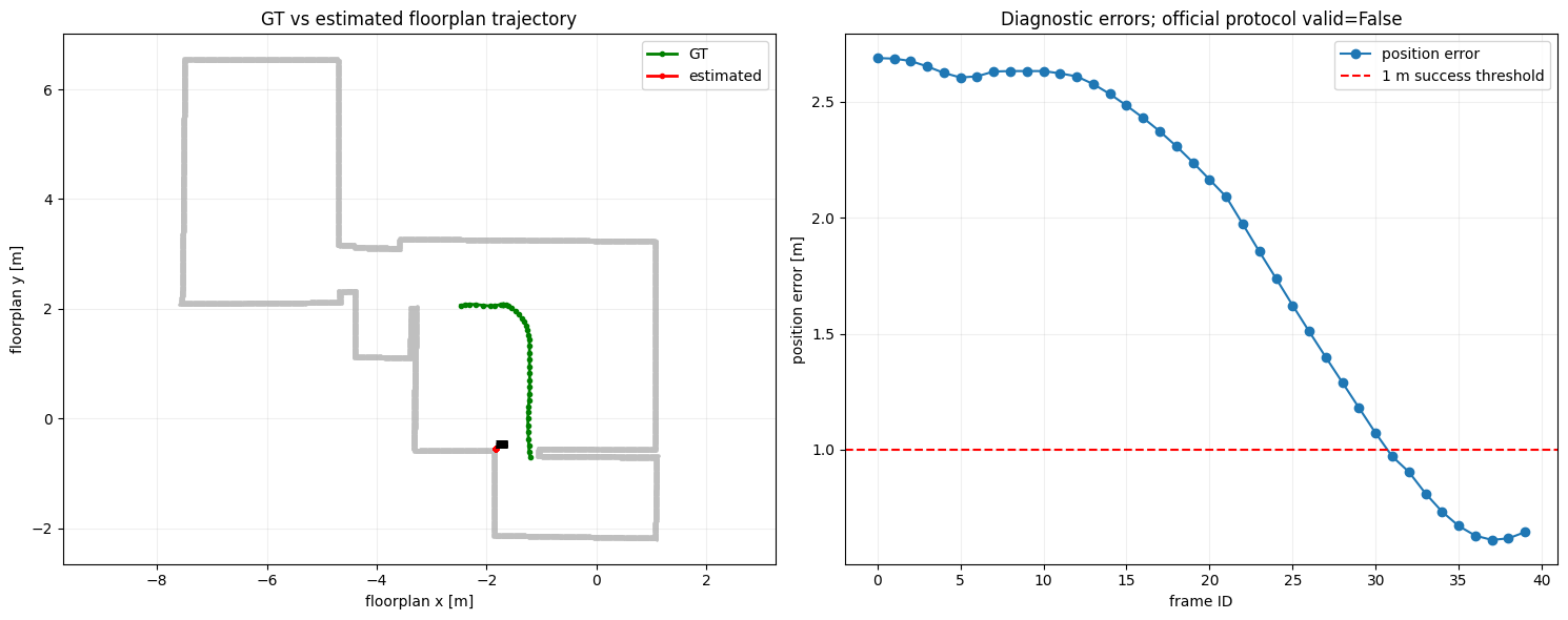
도면상에서 실제 카메라 Pose와 추정값 사이의 거리가 1m이내로 들어왔으므로 성공으로 판단하며, 이미지 30장즈음을 기점으로 성공 기준을 넘어선다.
GPU의 설정에서 약간의 오류가 있어 MapAnything이 CPU로 돌아갔는데, 대략 5분가량의 시간이 걸렸다. (이미지 40장 처리하는데)
이후의 Solver들의 수행시간은 매우 빠른 편이다만, 주피터 노트북으로 구현했기때문에 정확한 실행시간은 확인하기 어렵다. 다만 논문에 따르면 RANSAC iteration은 100~300정도로 수행했다고 한다. 초기에 빨리 수렴한다고. 적진 않은데.. 내가 수행한 실험에선 Seed 당 500회로 수행했는데도 빨리 수렴하진 않는것 같은데…
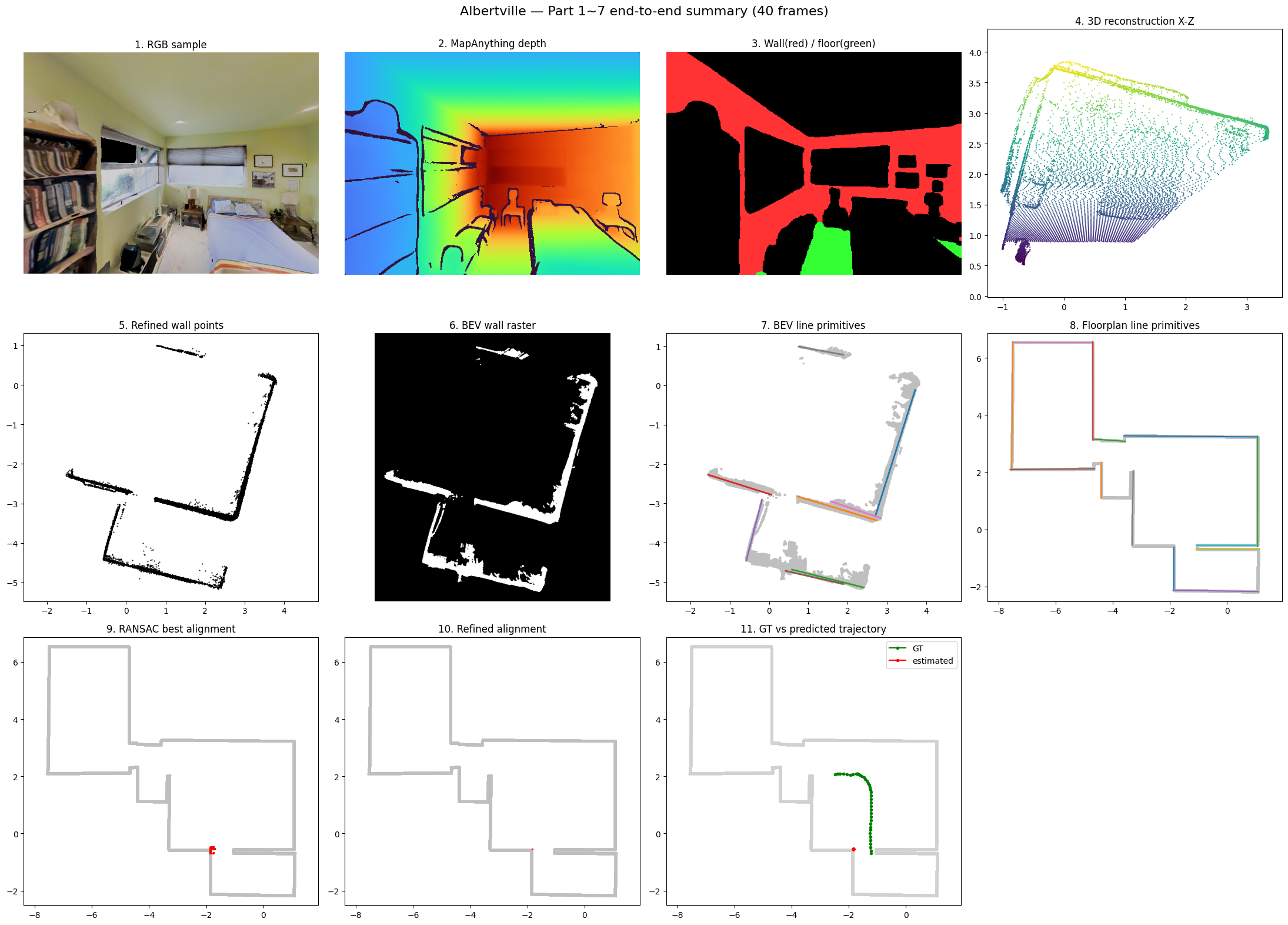
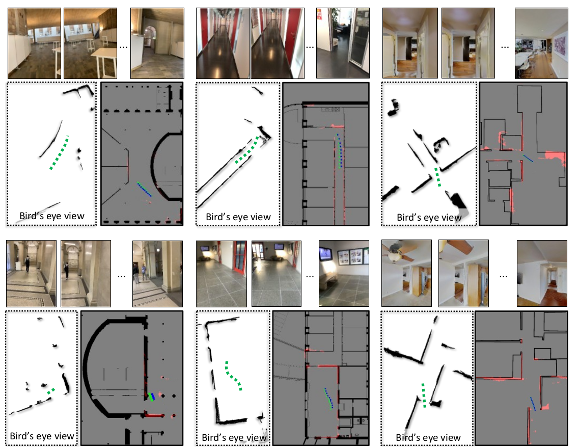
논문에선 좀더 복잡한 구조의 LaMAR데이터셋을 사용하여 수행했는데, 매칭도 잘되고, 짧은 trajectory 에서 성공율이 높다고 평가하고 있지만… 글쎄올시다…….. 하는 느낌도 없지 않다.
LaMAR HGE full에서 Z-FLoc은 ‘# 100’ 기준 SR@1m 83.6%를 기록했다. 같은 환경에서 학습된 UnLoc은 100.0%, F3Loc은 36.4%였다. UnLoc이 더 강한네.(이것도 Pollefey교수가 엮여있다) 즉 HGE 내부에서는 UnLoc이 더 높지만, Z-FLoc은 별도 학습 없이도 F3Loc보다 크게 높았음을 강조하는데, 이건 Unloc을 좀 해보고 나서 평가를 해야 할 것 같다.
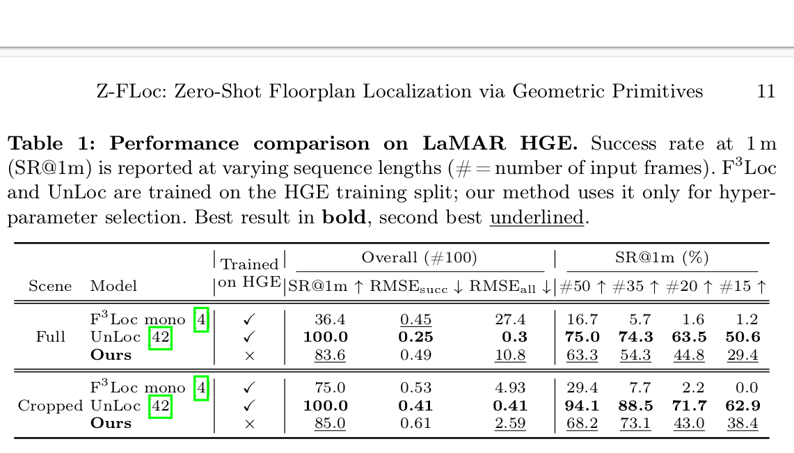
역시나 세밀한 위치추정은 Unloc쪽이 0.49m vs 0.25m로 더 우세한데, Geometry를 직접적으로 사용하는 알고리즘임에도 생각보다 오차가 크다는게 조금 신기하다. Unloc쪽을 읽어봐야 알겠지만, MapAnything의 출력 정밀도에 의존하게 되어 그런것 아닐까 하는 의심을 해본다.
다만 다른 논문들은 LaMAR HGE에서 학습한걸 LaMAR CABd으로 가져와 사용할 경우 결과가 폭망한다고 하는데, Z-Floc은 잘된다고 강조한다. 아무래도 Geometry 매칭을 특징으로 하니 그럴수밖에.
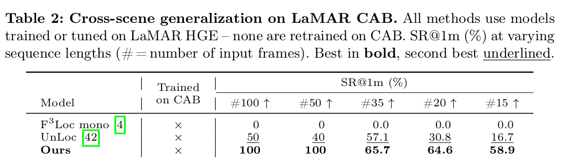
실험결과를 요약하면, 다음과 같다.
- 같은 환경에서 충분히 학습된 UnLoc이 더 강한 경우는 있다.
- 하지만 새로운 환경으로 넘어갈 때 Z-FLoc의 zero-shot generalization이 훨씬 안정적이다.
결론.
우선, 2D 캐드도면과, RGB만을 이용해 만든 3D 공간을 어떻게 매칭하는가에 대해 매우 좋은 아이디어를 제시한건 높이 평가 한다. 정말 아이디어가 좋았다. 선과 원을 추출하는 방법들과, 그것을 비교하는 방법에 있어서 수학적인 해법들은 정말 참신했다.
다만, 이 방법이 SOTA로 보기에는 어려운점은 아쉽다. 우선 퍼포먼스가 충분히 나오진 않는다는 것과, 다른 환경과 다른 도면에서 어떻게 수행될지 확실하지 않다는 것이 걱정된다.
특히 데이터셋들의 도면들이 매우 깔끔하게 정제되어있는데, 이런 도면을 얻지 못한다면 특징점 비교에 어려움이 있지 않을까 우려된다. 아마 필드 적용에선 이 단계부터 벽에 부딛히지 않을까 생각된다.
3D depth 추정까지 DL 모델에 의존하다보니 연산속도에 제약이 크고, 임베디드화에 걱정점이 있다. 마찬가지로 사물인식 역시 DL 모델을 사용하기에, GPU의 핸들링이나, 메모리 관리에서 주의를 요한다. 아.. 그러네.. 메모리 체크 못해봤다.. 이런 부분들은 RGBD센서를 이용한 3D reconstruction 알고리즘들을 사용하면 충분히 대체가능하지 않을까 하는 생각도 해본다.
벽을 추출하는 과정에서도 잘못된 벽을 날리는 방법이라던가, 문/통로의 처리 방식 자체는 참신한데, 실제로 했을 경우 유리창이 있을때 벽이 통째로 없어지는걸 봤다. 분명 잘못이긴 한데, 하긴.. 다른 2D도면에선 창문 기호가 있고, 이걸 벽으로 치환하는게 잘 안되기도 했다. 그걸 생각하면 차라리 창문을 지워버리고 뚫린 공간처럼 인식하는것도 의미는 있겠네…
덤으로, 논문 자체에 대한 것보다 논문에서 언급하는 여러 CV 관련 이론들이나 기하학 이론들, 그리고 Related work에서 소개된 논문들이 매우 도움이 되는 논문이다. 덕분에 논문 외적으로 많은 공부가 되었다.
9월 15일부터 리뷰페이지 작성을 시작해서, 무려 보름만에 작성을 마무리한다. 아따.. 길다. 끗.
댓글남기기